Tiling

Tiling for both raster and vector data

Tiler

 Tiler (outpath, gridsize_x:int=400, gridsize_y:int=400,
        overlap:Tuple[int,int]=(100, 100))

Similar functions than ´solaris.tile.raster_tile’ but with more recent dependencies.

source

Tiler.tile_raster

 Tiler.tile_raster (path_to_raster:str, allow_partial_data:bool=False)

Tiles specified raster to self.gridsize_x times self.gridsize_y grid, with self.overlap pixel overlap

source

Tiler.tile_vector

 Tiler.tile_vector (path_to_vector:str, min_area_pct:float=0.0)

Tiles a vector data file into smaller tiles. Converts all multipolygons to a regular polygons. min_area_pct is be used to specify the minimum area for partial masks to keep. Default value 0.0 keeps all masks.

source

Tiler.tile_and_rasterize_vector

 Tiler.tile_and_rasterize_vector (path_to_raster:str, path_to_vector:str,
                                  column:str, keep_bg_only:bool=False)

Rasterizes vectors based on tiled rasters. Requires that shapefile has numeric data in column. By default only keeps the patches that contain polygon data, by specifying keep_bg_only=True saves also masks for empty patches.

source

untile_vector

 untile_vector (path_to_targets:str, outpath:str,
                non_max_suppression_thresh:float=0.0,
                nms_criterion:str='score')

Create single shapefile from a directory of predicted shapefiles

source

copy_sum

 copy_sum (merged_data, new_data, merged_mask, new_mask, **kwargs)

Make new pixels have the sum of two overlapping pixels as their value. Useful with prediction data

source

untile_raster

 untile_raster (path_to_targets:str, outfile:str, method:str='first')

Merge multiple patches from path_to_targets into a single raster`

f = gpd.read_file('example_data/R70C21.shp')
f.head()
f['label_id'] = f.apply(lambda row: 2 if row.label == 'Standing' else 1, axis=1)
f.to_file('example_data/R70C21.shp')

Example area looks like this

from rasterio import plot as rioplot

raster = rio.open('example_data/R70C21.tif')
rioplot.show(raster)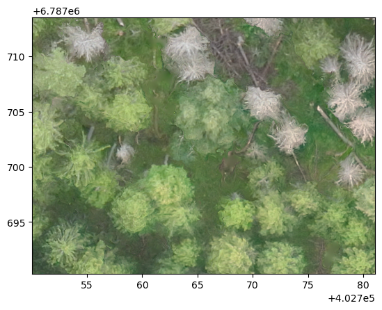

<Axes: >

With rasterio.plot it is a lot easier to visualize shapefile and raster simultaneously

fig, ax = plt.subplots(1,1)
rioplot.show(raster, ax=ax)
f.plot(ax=ax, column='label_id')

<Axes: >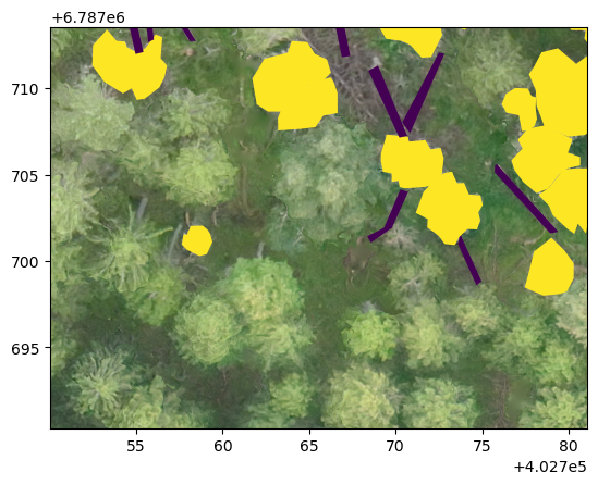

Let’s tile image into 240x180 sized patches using overlap of half patch size.

tiler = Tiler(outpath='example_data/tiles', gridsize_x=240, gridsize_y=180, overlap=(120, 90))

tiler.tile_raster('example_data/R70C21.tif')

tiler.tile_vector('example_data/R70C21.shp', min_area_pct=.2)

Untile shapefiles and check how they look

untile_vector(f'example_data/tiles/vectors', outpath='example_data/untiled.geojson')

81 polygons before non-max suppression
81 polygons after non-max suppression

Plot with the tiled grid.

untiled = gpd.read_file('example_data/untiled.geojson')
fig, ax = plt.subplots(1,1)
rioplot.show(raster, ax=ax)
tiler.grid.exterior.plot(ax=ax)
untiled.plot(ax=ax, column='label_id', facecolor='none', edgecolor='black')

<Axes: >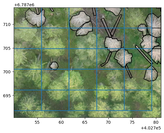

If allow_partial_data=False as is the default behaviour, tiling is done only for the area from which full sized patch can be extracted. With allow_partial_data=True, windows can “extend” to empty areas. This is useful with inference, when predicted areas can have wonky dimensions.

tiler.tile_raster('example_data/R70C21.tif', allow_partial_data=True)

tiler.tile_vector('example_data/R70C21.shp', min_area_pct=.2)

Untile shapefiles and check how they look

untile_vector(f'example_data/tiles/vectors', outpath='example_data/untiled.geojson')

81 polygons before non-max suppression
81 polygons after non-max suppression

untiled = gpd.read_file('example_data/untiled.geojson')
fig, ax = plt.subplots(1,1)
rioplot.show(raster, ax=ax)
#tiler.grid.exterior.plot(ax=ax)
untiled.plot(ax=ax, column='label_id', facecolor='none', edgecolor='black')

<Axes: >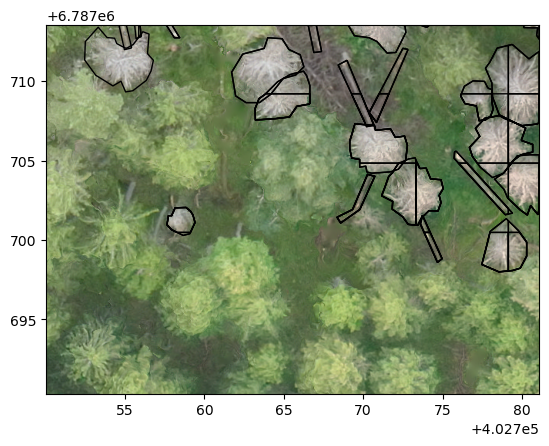

Plot with the tiled grid.

untiled = gpd.read_file('example_data/untiled.geojson')
fig, ax = plt.subplots(1,1)
rioplot.show(raster, ax=ax)
tiler.grid.exterior.plot(ax=ax)
untiled.plot(ax=ax, column='label_id')

<Axes: >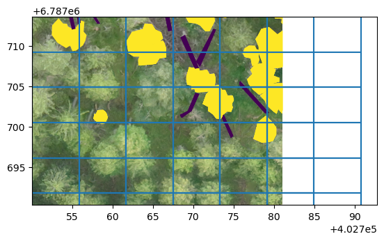

tiler.tile_and_rasterize_vector('example_data/R70C21.tif', 'example_data/R70C21.shp', column='label_id')

tiler.tile_and_rasterize_vector('example_data/R70C21.tif', 'example_data/R70C21.shp', 
                                column='label_id', keep_bg_only=True)

import matplotlib.pyplot as plt

with rio.open('example_data/tiles/rasterized_vectors/R1C3.tif') as i: im = i.read()
plt.imshow(im[0])

<matplotlib.image.AxesImage>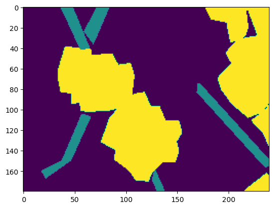

untile_raster can be used to mosaic all patches into one.

untile_raster('example_data/tiles/rasterized_vectors/', 'example_data/tiles/mosaic_first.tif', 
              method='first')

with rio.open('example_data/tiles/mosaic_first.tif') as mos: mosaic = mos.read()
plt.imshow(mosaic[0])

<matplotlib.image.AxesImage>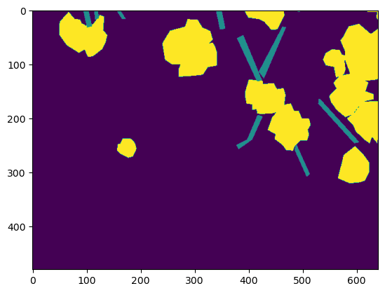

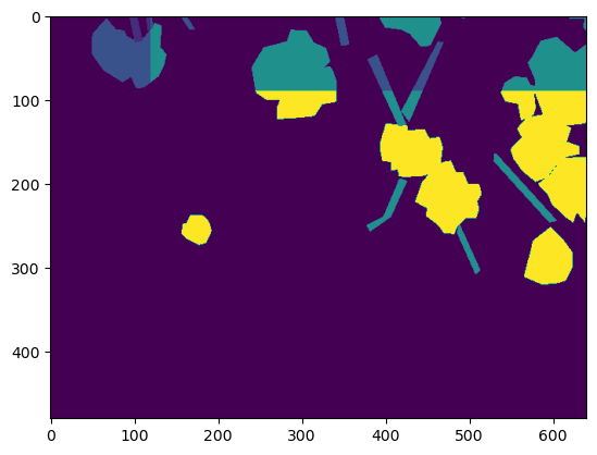
By specifying method as sum it’s possible to collate predictions and get the most likely label for pixels

untile_raster('example_data/tiles/rasterized_vectors/', 'example_data/tiles/mosaic_sum.tif',
              method='sum')

with rio.open('example_data/tiles/mosaic_sum.tif') as mos: mosaic = mos.read()
plt.imshow(mosaic[0])

<matplotlib.image.AxesImage>