Tabular data workflow

Point-based

import rasterio as rio
import geopandas as gpd
from pathlib import Path
import rasterio.plot as rioplot
import matplotlib.pyplot as plt

path_to_data = Path('workflow_examples/')
raster_data = path_to_data/'s2_2018_lataseno.tif'
point_data = path_to_data/'points_clc.geojson'

Example data here are Sentinel 2 mosaic from 2018, with 9 bands, and scattered point observations from that area. Target class for the points is Corine Land Cover class for the corresponding location

fig, axs = plt.subplots(1,2, dpi=100, figsize=(10,4))
with rio.open(raster_data) as src:
    rioplot.show((src, (3,2,1)), adjust=True, ax=axs[0])
train_gdf = gpd.read_file(point_data)
train_gdf['corine'] = train_gdf.corine.astype('category')
train_gdf.plot(column='corine', ax=axs[1], cmap='tab20', markersize=1, legend=True,
               legend_kwds={'loc':'right', 'bbox_to_anchor':(1.2,0.5)})
plt.suptitle('Example area')
plt.tight_layout()
plt.show()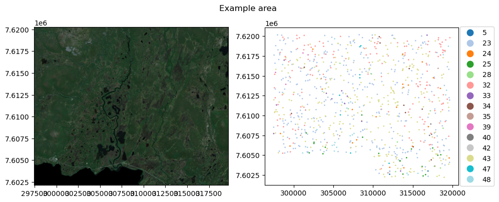

Create the dataset

CLI

geo2ml_sample_points \
example_data/workflow_examples/points_clc.geojson \
example_data/workflow_examples/s2_2018_lataseno.tif \
corine \
example_data/workflow_examples/points/ \
--out_prefix example

Python

from geo2ml.scripts.data import sample_points

outpath = path_to_data/'points'

sample_points(point_data, raster_data, 'corine', outpath, out_prefix='example')

Training a random forest

from sklearn.ensemble import RandomForestClassifier
from sklearn.metrics import classification_report
from sklearn.model_selection import train_test_split
import pandas as pd

df = pd.read_csv(outpath/'example__s2_2018_lataseno__points_clc__corine.csv')

y = df['corine']
X = df.drop(columns='corine')

X_train, X_test, y_train, y_test = train_test_split(X, y)

rf = RandomForestClassifier()
rf.fit(X_train, y_train)

RandomForestClassifier()

In a Jupyter environment, please rerun this cell to show the HTML representation or trust the notebook.
On GitHub, the HTML representation is unable to render, please try loading this page with nbviewer.org.

y_pred = rf.predict(X_test)
print(classification_report(y_test, y_pred, zero_division=0))

              precision    recall  f1-score   support

          23       0.55      0.77      0.64        81
          24       0.00      0.00      0.00         7
          25       0.00      0.00      0.00         7
          28       0.00      0.00      0.00         2
          32       0.42      0.36      0.39        36
          33       0.00      0.00      0.00         2
          34       0.00      0.00      0.00         2
          35       0.00      0.00      0.00         3
          39       0.00      0.00      0.00         1
          40       0.00      0.00      0.00         2
          42       0.00      0.00      0.00         1
          43       0.70      0.72      0.71        75
          47       1.00      0.50      0.67         2
          48       0.83      0.83      0.83         6

    accuracy                           0.59       227
   macro avg       0.25      0.23      0.23       227
weighted avg       0.53      0.59      0.55       227

Polygon-based

Example data here is RGB UAV data from Evo, Hämeenlinna, and the target polygons are tree canopies. Target class is the species (Spruce, pine, birch, aspen) or standing deadwood, found on column label. As the extracted features, we use min, max, mean, std and median of the red, green and blue channels within the canopies.

uav_data = path_to_data/'example_area.tif'
canopy_data = path_to_data/'canopies.geojson'

fig, axs = plt.subplots(1,2, dpi=100, figsize=(5,7))
with rio.open(uav_data) as src:
    rioplot.show((src, (1,2,3)), adjust=True, ax=axs[0])
train_gdf = gpd.read_file(canopy_data)
train_gdf.plot(column='label', ax=axs[1], cmap='tab20')
plt.suptitle('Example area')
plt.tight_layout()
plt.show()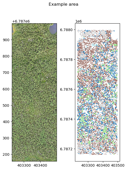

CLI

geo2ml_sample_polygons \
example_data/workflow_examples/canopies.geojson \
example_data/workflow_examples/example_area.tif \
label \
example_data/workflow_examples/polygons/ \
--out_prefix example \
--min --max --mean --std --median

Python

from geo2ml.scripts.data import sample_polygons

outpath = path_to_data/'polygons'

sample_polygons(canopy_data, uav_data, 'label', outpath, out_prefix='example',
                min=True, max=True, mean=True, std=True, median=True,
                count=False, sum=False, categorical=False)

/home/mayrajeo/miniconda3/envs/point-eo-dev/lib/python3.11/site-packages/rasterstats/io.py:328: NodataWarning: Setting nodata to -999; specify nodata explicitly
  warnings.warn(

Dataset structure

Train model

from sklearn.preprocessing import LabelEncoder
from sklearn.metrics import confusion_matrix, ConfusionMatrixDisplay

df = pd.read_csv(outpath/'example__example_area__canopies__label.csv')

le = LabelEncoder()
y = le.fit_transform(df['label'])
X = df.drop(columns='label')

X_train, X_test, y_train, y_test = train_test_split(X, y)

rf = RandomForestClassifier()
rf.fit(X_train, y_train)

RandomForestClassifier()

y_pred = rf.predict(X_test)
print(classification_report(y_test, y_pred, zero_division=0, target_names=le.classes_))

                   precision    recall  f1-score   support

            Birch       0.67      0.59      0.63       326
   European aspen       0.85      0.50      0.63       102
    Norway spruce       0.83      0.93      0.87       777
       Scots pine       0.84      0.78      0.81       273
Standing deadwood       0.96      0.96      0.96        74

         accuracy                           0.81      1552
        macro avg       0.83      0.75      0.78      1552
     weighted avg       0.80      0.81      0.80      1552

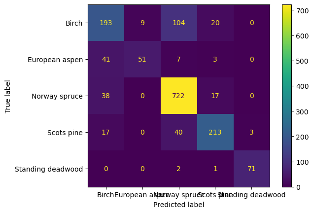
cm = confusion_matrix(y_test, y_pred, labels=rf.classes_)
disp = ConfusionMatrixDisplay(confusion_matrix=cm, display_labels=le.classes_)
disp.plot()
plt.show()