After post-processing the results, we used them do derive land use and land cover changes for our study area.
Change analyses
Change analyses can be done with either raster data or polygon data. Working with polygon data is much easier, as newer topographical databases are also polygon data.
Code
def polygonize(fn, outpath, target_class, scale_factor= 1 ):with rio.open (fn) as src:= src.read(out_shape= (src.count, int (src.height* scale_factor),int (src.width* scale_factor)),= Resampling.mode)[target_class - 1 ]!= 0 ] = 1 = im == 1 = src.transform * src.transform.scale((src.width/ im.shape[- 1 ]), (src.height/ im.shape[- 2 ]))= ({'properties' : {'raster_val' : v}, 'geometry' : s}for i, (s, v) in enumerate (features.shapes(im, mask== mask, transform= tfm))if v == 1 )with fiona.open (outpath, 'w' , driver= 'GeoJSON' ,= 'EPSG:3067' ,= {'properties' : [('raster_val' , 'int' )],'geometry' : 'Polygon' }) as dst:
Also, as the maps are not perfectly aligned, the analysis is done by aggregating the data into a rectangular grid.
Code
def make_grid(area, cell):= area.total_bounds= list (np.arange(xmin, xmax+ cell, cell))= list (np.arange(ymin, ymax+ cell, cell))= []= []for (C,x), (R,y) in product(enumerate (cols[:- 1 ]), enumerate (rows[:- 1 ])):+ cell, y), (x+ cell,y+ cell),(x, y+ cell)]))f'R { R} C { C} ' )return gpd.GeoDataFrame({'geometry' :polys, 'cellid' :names}, crs= area.crs)
Code
= Path('../results/processed/' )= os.listdir(respath)
Fields
First polygonize the results.
Code
= Path('../results/polygons/' )for r in results:/ r, polypath/ 'fields' / r.replace('tif' , 'geojson' ), target_class= 1 , scale_factor= 1 / 2 )
Then put them into a single dataframe
Code
= None = None for p in os.listdir(polypath/ 'fields' ):= gpd.read_file(polypath/ 'fields' / p)if '1965' in p:if fields_65 is None : fields_65 = union_gdfelse : fields_65 = pd.concat((fields_65, union_gdf))else :if fields_80s is None : fields_80s = union_gdfelse : fields_80s = pd.concat((fields_80s, union_gdf))= fields_65.clip(study_area.geometry.iloc[0 ])= fields_80s.clip(study_area.geometry.iloc[0 ])= True , drop= True )= True , drop= True )
Save the dataframes.
Code
/ 'fields_65.geojson' )/ 'fields_80s.geojson' )
Code
= gpd.read_file(mtk_path/ '2005/fields.geojson' )= gpd.read_file(mtk_path/ '2022/pellot_2022.geojson' )
Code
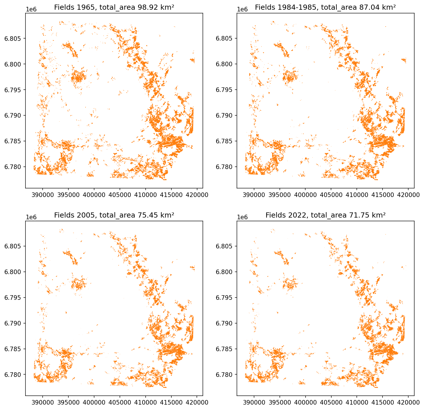
= plt.subplots(2 ,2 , figsize= (10 ,10 ), dpi= 150 )= axs[0 ,0 ], color= 'tab:orange' )0 ,0 ].set_title(f'Fields 1965, total_area { (fields_65.area.sum () * 10 **- 6 ):.2f} km²' )= axs[0 ,1 ], color= 'tab:orange' )0 ,1 ].set_title(f'Fields 1984-1985, total_area { (fields_80s.area.sum () * 10 **- 6 ):.2f} km²' )= axs[1 ,0 ], color= 'tab:orange' )1 ,0 ].set_title(f'Fields 2005, total_area { (fields_05.area.sum () * 10 **- 6 ):.2f} km²' )= axs[1 ,1 ], color= 'tab:orange' )1 ,1 ].set_title(f'Fields 2022, total_area { (fields_22.area.sum () * 10 **- 6 ):.2f} km²' )
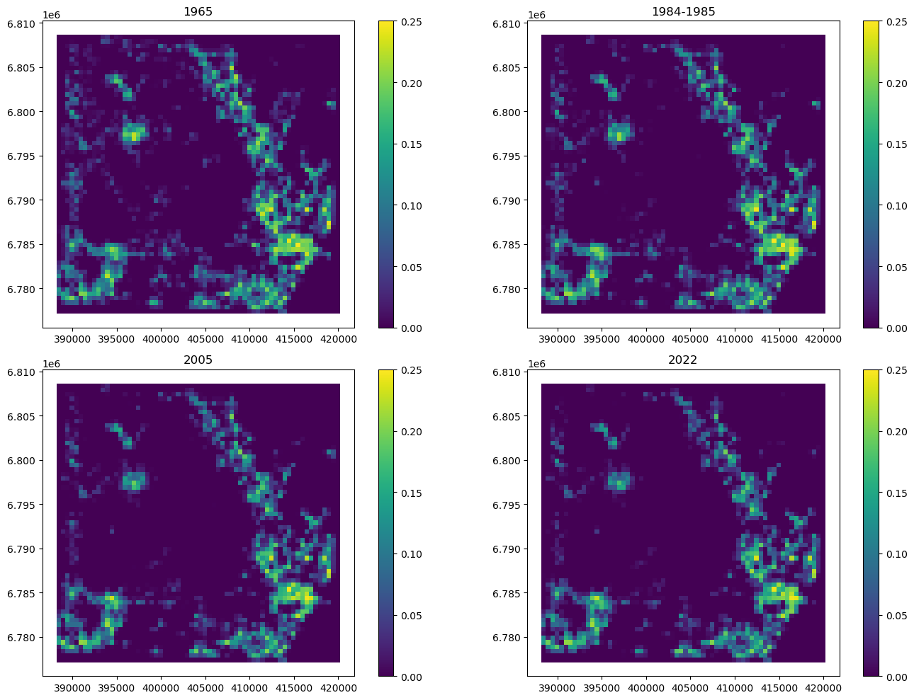
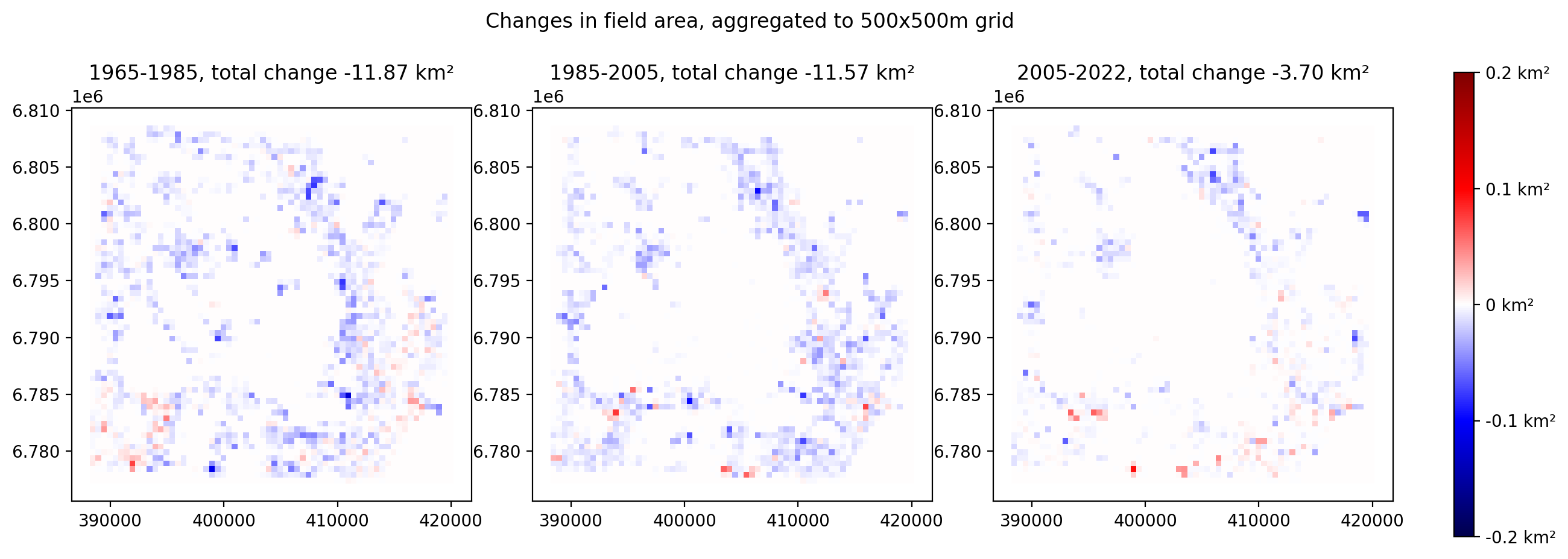
From 1965 to 2022, the total field area has decreased by around 30 km². However, visualizing where the change has been most significant is rather difficult from the polygon data, so we aggregate the data into 500x500m grid.
Code
def aggregate_area_to_grid(grid, polys, column_name):= grid[['cellid' , 'geometry' ]].copy()= tempgrid.overlay(polys, how= 'intersection' ).dissolve(by= 'cellid' ).reset_index(drop= False )= tempgrid.geometry.area * 10 **- 6 = grid.merge(tempgrid[['cellid' , column_name]], how= 'left' , on= 'cellid' )return grid
Code
= make_grid(study_area, 500 )
Code
= aggregate_area_to_grid(grid, fields_65, 'field_area_65' )= aggregate_area_to_grid(grid, fields_80s, 'field_area_85' )= aggregate_area_to_grid(grid, fields_05, 'field_area_05' )= aggregate_area_to_grid(grid, fields_22, 'field_area_22' )
Code
= plt.subplots(2 ,2 , figsize= (14 ,10 ))0 , inplace= True )= 'field_area_65' , ax= axs[0 ,0 ], vmin= 0 , vmax= .500 ** 2 , legend= True ).set_title('1965' )= 'field_area_85' , ax= axs[0 ,1 ], vmin= 0 , vmax= .500 ** 2 , legend= True ).set_title('1984-1985' )= 'field_area_05' , ax= axs[1 ,0 ], vmin= 0 , vmax= .500 ** 2 , legend= True ).set_title('2005' )= 'field_area_22' , ax= axs[1 ,1 ], vmin= 0 , vmax= .500 ** 2 , legend= True ).set_title('2022' )
Quantify the change. Negative change means decreased field area.
Code
'field_change_6585' ] = (grid.field_area_85 - grid.field_area_65)'field_change_8505' ] = (grid.field_area_05 - grid.field_area_85)'field_change_0522' ] = (grid.field_area_22 - grid.field_area_05)
Change stats for 1965-1985:
Code
print (f'Gain: { grid[grid.field_change_6585 > 0 ]. field_change_6585. sum ():.2f} km²' )print (f'Loss: { - grid[grid.field_change_6585 < 0 ]. field_change_6585. sum ():.2f} km²' )print (f'Change: { grid. field_change_6585. sum ():.2f} km²' )
Gain: 2.32 km²
Loss: 14.20 km²
Change: -11.87 km²
Change stats for 1985-2005
Code
print (f'Gain: { grid[grid.field_change_8505 > 0 ]. field_change_8505. sum ():.2f} km²' )print (f'Loss: { - grid[grid.field_change_8505 < 0 ]. field_change_8505. sum ():.2f} km²' )print (f'Change: { grid. field_change_8505. sum ():.2f} km²' )
Gain: 1.27 km²
Loss: 12.85 km²
Change: -11.57 km²
Change stats for 2005-2022
Code
print (f'Gain: { grid[grid.field_change_0522 > 0 ]. field_change_0522. sum ():.2f} km²' )print (f'Loss: { - grid[grid.field_change_0522 < 0 ]. field_change_0522. sum ():.2f} km²' )print (f'Change: { grid. field_change_0522. sum ():.2f} km²' )
Gain: 1.81 km²
Loss: 5.51 km²
Change: -3.70 km²
Code
= plt.subplots(1 ,4 , figsize= (15 ,5 ), dpi= 200 , gridspec_kw= {'width_ratios' : [1 ,1 ,1 ,0.05 ]})= 'field_change_6585' , cmap= 'seismic' , vmin=- .20 , vmax= .20 , ax= axs[0 ])= 'field_change_8505' , cmap= 'seismic' , vmin=- .20 , vmax= .20 , ax= axs[1 ])= 'field_change_0522' , cmap= 'seismic' , vmin=- .20 , vmax= .20 , ax= axs[2 ])0 ].set_title(f'1965-1985, total change { grid. field_change_6585. sum ():.2f} km²' )1 ].set_title(f'1985-2005, total change { grid. field_change_8505. sum ():.2f} km²' )2 ].set_title(f'2005-2022, total change { grid. field_change_0522. sum ():.2f} km²' )= colors.Normalize(vmin=- .2 ,vmax= .2 )= plt.cm.ScalarMappable(cmap= 'seismic' , norm= norm)= [- .2 ,- .1 ,0 ,.1 ,.2 ]= plt.colorbar(sm, cax= axs[3 ], ticks= ticks)f' { t} km²' for t in ticks])'Changes in field area, aggregated to 500x500m grid' )
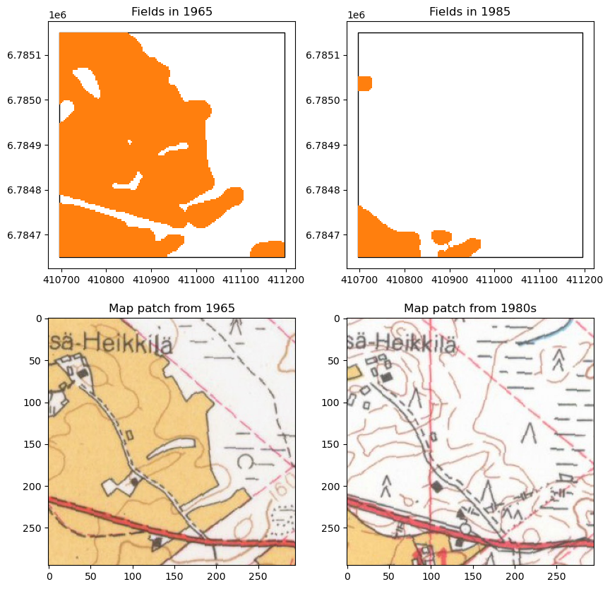
Visualize the location where the field area has decreased the most between 1965 and 1985. For 1965 and 1980s show the corresponding map patch along with the data.
Code
from shapely.geometry import boxfrom rasterio.windows import from_boundsdef get_map_patch(bbox, year, map_path):"Get map patch to go along with the desired location" if year == 1965 : files = [f for f in os.listdir(map_path) if '1965' in f]else : files = [f for f in os.listdir(map_path) if '1965' not in f]for f in files:with rio.open (map_path/ f) as src:= src.boundsif not bbox.within(box(* tot_bounds)): continue = src.read(window= from_bounds(* bbox.bounds, src.transform))return np.moveaxis(data, 0 , 2 )
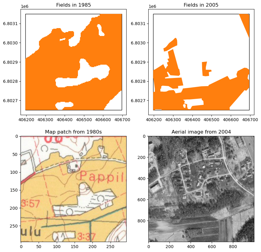
For 2005 and 2022, show the closest aerial image to that year. Unfortunately the closest historical images available are from 1949 and 1979, so we can’t really use them for visualizations.
Code
import owslib.wcs as wcsimport iodef get_wcs_img(bounds, year):= 'https://beta-karttakuva.maanmittauslaitos.fi/ortokuvat-ja-korkeusmallit/wcs/v1' = wcs.WebCoverageService(mml_wcs_url)#, version='2.0.1') = year= 0 while True :if year < 2009 : layer = 'ortokuva_mustavalko' else : layer = 'ortokuva_vari' = mml_wcs.getCoverage(identifier= [layer],= 'EPSG:3067' ,= [('E' , bounds[0 ], bounds[2 ]), 'N' , bounds[1 ], bounds[3 ]), 'time' , f' { year} -12-31T00:00:00.000Z' )],format = 'image/tiff' )= io.BytesIO(img_rgb.read())with rio.open (image) as src:= src.read()if data.max () != data.min (): break += 1 = year - tries if tries% 2 == 0 else year + tries= year return np.moveaxis(data, 0 , 2 ), finalyear
Code
= Path('../data/maps/aligned_maps/' )= grid[grid.field_change_6585 == grid.field_change_6585.min ()].cellid.iloc[0 ]= plt.subplots(2 ,2 , figsize= (10 ,10 ))== fieldloss_6585_cellid].plot(ax= axs[0 ,0 ], facecolor= 'none' )== fieldloss_6585_cellid].geometry).plot(ax= axs[0 ,0 ], color= 'tab:orange' ).set_title('Fields in 1965' )== fieldloss_6585_cellid].plot(ax= axs[0 ,1 ], facecolor= 'none' )== fieldloss_6585_cellid].geometry).plot(ax= axs[0 ,1 ], color= 'tab:orange' ).set_title('Fields in 1985' )= get_map_patch(grid[grid.cellid == fieldloss_6585_cellid].geometry.iloc[0 ], 1965 , map_path)1 ,0 ].imshow(img, cmap= 'gray' )1 ,0 ].set_title(f'Map patch from 1965' )= get_map_patch(grid[grid.cellid == fieldloss_6585_cellid].geometry.iloc[0 ], 1985 , map_path)1 ,1 ].imshow(img, cmap= 'gray' )1 ,1 ].set_title(f'Map patch from 1980s' )
Same for 1985 and 2005
Code
= grid[grid.field_change_8505 == grid.field_change_8505.min ()].cellid.iloc[0 ]= plt.subplots(2 ,2 , figsize= (10 ,10 ))== fieldloss_8505_cellid].plot(ax= axs[0 ,0 ], facecolor= 'none' )== fieldloss_8505_cellid].geometry).plot(ax= axs[0 ,0 ], color= 'tab:orange' ).set_title('Fields in 1985' )== fieldloss_8505_cellid].plot(ax= axs[0 ,1 ], facecolor= 'none' )== fieldloss_8505_cellid].geometry).plot(ax= axs[0 ,1 ], color= 'tab:orange' ).set_title('Fields in 2005' )= get_map_patch(grid[grid.cellid == fieldloss_8505_cellid].geometry.iloc[0 ], 1985 , map_path)1 ,0 ].imshow(img, cmap= 'gray' )1 ,0 ].set_title(f'Map patch from 1980s' )= get_wcs_img(grid[grid.cellid == fieldloss_8505_cellid].total_bounds, 2005 )1 ,1 ].imshow(img, cmap= 'gray' )1 ,1 ].set_title(f'Aerial image from { year} ' )
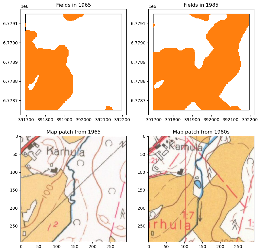
And then same visualizations for field area increase.
Code
= grid[grid.field_change_6585 == grid.field_change_6585.max ()].cellid.iloc[0 ]= plt.subplots(2 ,2 , figsize= (10 ,10 ))== fieldgain_6585_cellid].plot(ax= axs[0 ,0 ], facecolor= 'none' )== fieldgain_6585_cellid].geometry).plot(ax= axs[0 ,0 ], color= 'tab:orange' ).set_title('Fields in 1965' )== fieldgain_6585_cellid].plot(ax= axs[0 ,1 ], facecolor= 'none' )== fieldgain_6585_cellid].geometry).plot(ax= axs[0 ,1 ], color= 'tab:orange' ).set_title('Fields in 1985' )= get_map_patch(grid[grid.cellid == fieldgain_6585_cellid].geometry.iloc[0 ], 1965 , map_path)1 ,0 ].imshow(img, cmap= 'gray' )1 ,0 ].set_title(f'Map patch from 1965' )= get_map_patch(grid[grid.cellid == fieldgain_6585_cellid].geometry.iloc[0 ], 1985 , map_path)1 ,1 ].imshow(img, cmap= 'gray' )1 ,1 ].set_title(f'Map patch from 1980s' )
Code
= grid[grid.field_change_8505 == grid.field_change_8505.max ()].cellid.iloc[0 ]= plt.subplots(2 ,2 , figsize= (10 ,10 ))== fieldgain_8505_cellid].plot(ax= axs[0 ,0 ], facecolor= 'none' )== fieldgain_8505_cellid].geometry).plot(ax= axs[0 ,0 ], color= 'tab:orange' ).set_title('Fields in 1985' )== fieldgain_8505_cellid].plot(ax= axs[0 ,1 ], facecolor= 'none' )== fieldgain_8505_cellid].geometry).plot(ax= axs[0 ,1 ], color= 'tab:orange' ).set_title('Fields in 2005' )= get_map_patch(grid[grid.cellid == fieldgain_8505_cellid].geometry.iloc[0 ], 1985 , map_path)1 ,0 ].imshow(img, cmap= 'gray' )1 ,0 ].set_title(f'Map patch from 1980s' )= get_wcs_img(grid[grid.cellid == fieldgain_8505_cellid].total_bounds, 2005 )1 ,1 ].imshow(img, cmap= 'gray' )1 ,1 ].set_title(f'Aerial image from { year} ' )
Mires
Polygonize and put to single geojson files.
Code
for r in results:/ r, polypath/ 'mires' / r.replace('tif' , 'geojson' ), target_class= 2 , scale_factor= 1 / 2 )
Code
= None = None for p in os.listdir(polypath/ 'mires' ):= gpd.read_file(polypath/ 'mires' / p)if '1965' in p:if mires_65 is None : mires_65 = union_gdfelse : mires_65 = pd.concat((mires_65, union_gdf))else :if mires_80s is None : mires_80s = union_gdfelse : mires_80s = pd.concat((mires_80s, union_gdf))= mires_65.clip(study_area.geometry.iloc[0 ])= mires_80s.clip(study_area.geometry.iloc[0 ])= True , drop= True )= True , drop= True )
Code
/ 'mires_65.geojson' )/ 'mires_80s.geojson' )
Code
= gpd.read_file(mtk_path/ '2005/mires.geojson' )= gpd.read_file(mtk_path/ '2022/suot_2022.geojson' )
Code
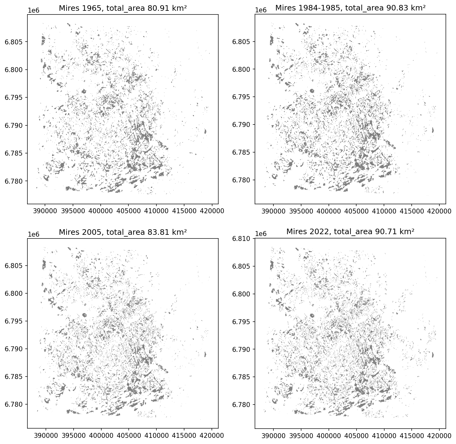
= plt.subplots(2 ,2 , figsize= (10 ,10 ), dpi= 150 )= axs[0 ,0 ], color= 'tab:gray' )0 ,0 ].set_title(f'Mires 1965, total_area { (mires_65.area.sum () * 10 **- 6 ):.2f} km²' )= axs[0 ,1 ], color= 'tab:gray' )0 ,1 ].set_title(f'Mires 1984-1985, total_area { (mires_80s.area.sum () * 10 **- 6 ):.2f} km²' )= axs[1 ,0 ], color= 'tab:gray' )1 ,0 ].set_title(f'Mires 2005, total_area { (mires_05.area.sum () * 10 **- 6 ):.2f} km²' )= axs[1 ,1 ], color= 'tab:gray' )1 ,1 ].set_title(f'Mires 2022, total_area { (mires_22.area.sum () * 10 **- 6 ):.2f} km²' )
The difference between the total areas of mires between years can be explained by more accurate mapping methods, or restoration processes.
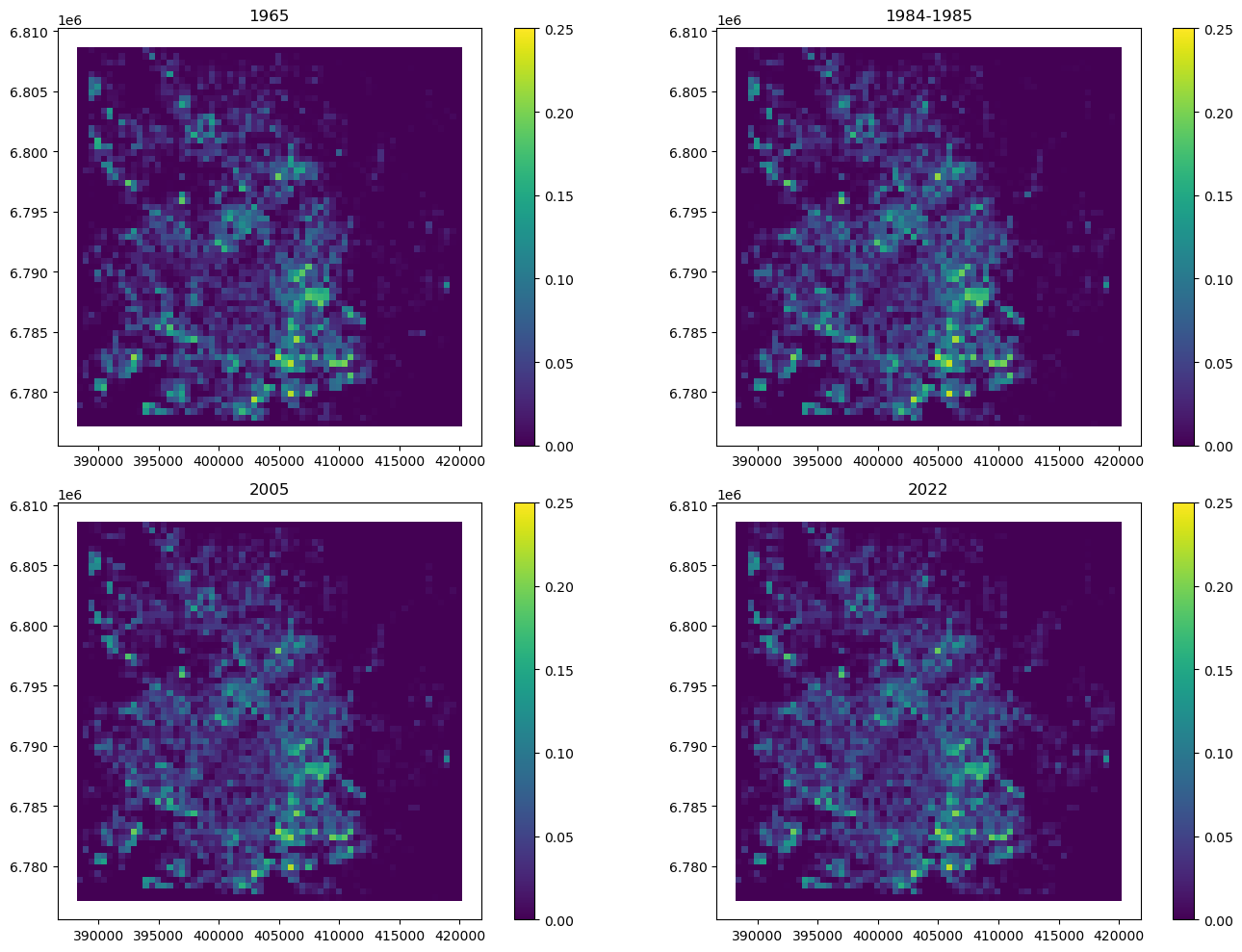
Put the data into the grid.
Code
= aggregate_area_to_grid(grid, mires_65, 'mire_area_65' )= aggregate_area_to_grid(grid, mires_80s, 'mire_area_85' )= aggregate_area_to_grid(grid, mires_05, 'mire_area_05' )= aggregate_area_to_grid(grid, mires_22, 'mire_area_22' )
Code
= plt.subplots(2 ,2 , figsize= (14 ,10 ))0 , inplace= True )= 'mire_area_65' , ax= axs[0 ,0 ], vmin= 0 , vmax= .500 ** 2 , legend= True ).set_title('1965' )= 'mire_area_85' , ax= axs[0 ,1 ], vmin= 0 , vmax= .500 ** 2 , legend= True ).set_title('1984-1985' )= 'mire_area_05' , ax= axs[1 ,0 ], vmin= 0 , vmax= .500 ** 2 , legend= True ).set_title('2005' )= 'mire_area_22' , ax= axs[1 ,1 ], vmin= 0 , vmax= .500 ** 2 , legend= True ).set_title('2022' )
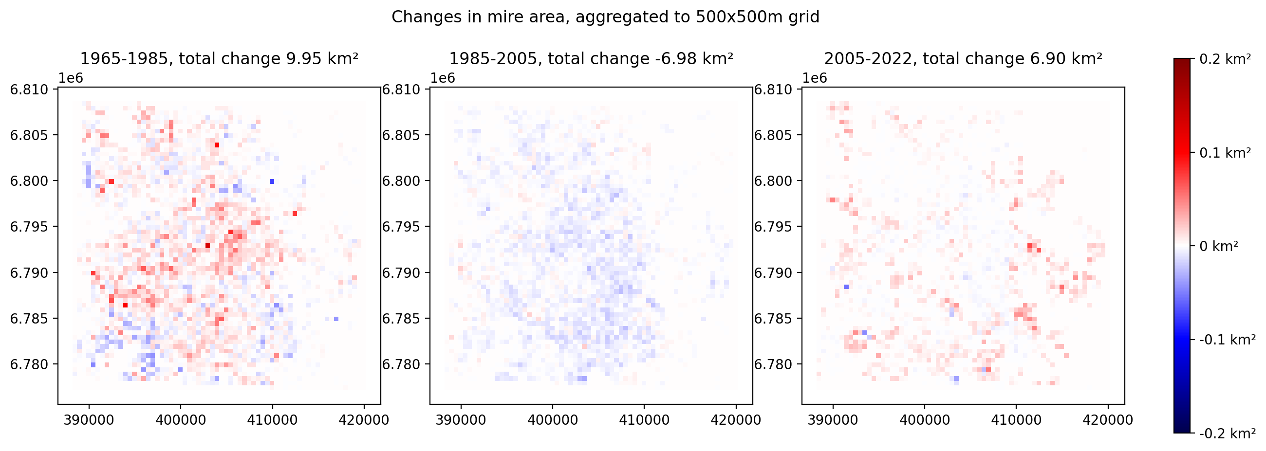
Quantify the change. Negative change means decreased mire area.
Code
'mire_change_6585' ] = (grid.mire_area_85 - grid.mire_area_65)'mire_change_8505' ] = (grid.mire_area_05 - grid.mire_area_85)'mire_change_0522' ] = (grid.mire_area_22 - grid.mire_area_05)
Change stats for 1965-1985:
Code
print (f'Gain: { grid[grid.mire_change_6585 > 0 ]. mire_change_6585. sum ():.2f} km²' )print (f'Loss: { - grid[grid.mire_change_6585 < 0 ]. mire_change_6585. sum ():.2f} km²' )print (f'Change: { grid. mire_change_6585. sum ():.2f} km²' )
Gain: 15.86 km²
Loss: 5.92 km²
Change: 9.95 km²
Change stats for 1985-2005
Code
print (f'Gain: { grid[grid.mire_change_8505 > 0 ]. mire_change_8505. sum ():.2f} km²' )print (f'Loss: { - grid[grid.mire_change_8505 < 0 ]. mire_change_8505. sum ():.2f} km²' )print (f'Change: { grid. mire_change_8505. sum ():.2f} km²' )
Gain: 1.74 km²
Loss: 8.72 km²
Change: -6.98 km²
Change stats for 2005-2022
Code
print (f'Gain: { grid[grid.mire_change_0522 > 0 ]. mire_change_0522. sum ():.2f} km²' )print (f'Loss: { - grid[grid.mire_change_0522 < 0 ]. mire_change_0522. sum ():.2f} km²' )print (f'Change: { grid. mire_change_0522. sum ():.2f} km²' )
Gain: 8.04 km²
Loss: 1.14 km²
Change: 6.90 km²
Code
= plt.subplots(1 ,4 , figsize= (15 ,5 ), dpi= 200 , gridspec_kw= {'width_ratios' : [1 ,1 ,1 ,0.05 ]})= 'mire_change_6585' , cmap= 'seismic' , vmin=- .20 , vmax= .20 , ax= axs[0 ])= 'mire_change_8505' , cmap= 'seismic' , vmin=- .20 , vmax= .20 , ax= axs[1 ])= 'mire_change_0522' , cmap= 'seismic' , vmin=- .20 , vmax= .20 , ax= axs[2 ])0 ].set_title(f'1965-1985, total change { grid. mire_change_6585. sum ():.2f} km²' )1 ].set_title(f'1985-2005, total change { grid. mire_change_8505. sum ():.2f} km²' )2 ].set_title(f'2005-2022, total change { grid. mire_change_0522. sum ():.2f} km²' )= colors.Normalize(vmin=- .2 ,vmax= .2 )= plt.cm.ScalarMappable(cmap= 'seismic' , norm= norm)= [- .2 ,- .1 ,0 ,.1 ,.2 ]= plt.colorbar(sm, cax= axs[3 ], ticks= ticks)f' { t} km²' for t in ticks])'Changes in mire area, aggregated to 500x500m grid' )
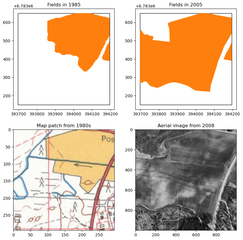
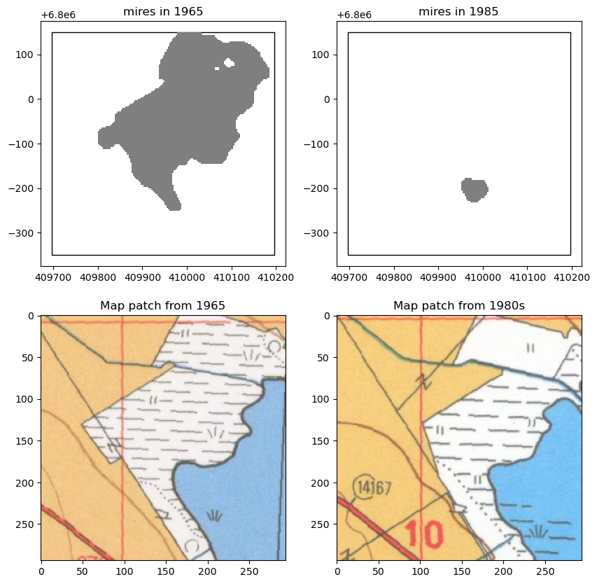
Visualize the location where the mire area has decreased the most between 1965 and 1985. For 1965 and 1980s show the corresponding map patch along with the data.
For 2005 and 2022, show the closest aerial image to that year. Unfortunately the closest historical images available are from 1949 and 1979, so we can’t really use them for visualizations.
Code
= grid[grid.mire_change_6585 == grid.mire_change_6585.min ()].cellid.iloc[0 ]= plt.subplots(2 ,2 , figsize= (10 ,10 ))== mireloss_6585_cellid].plot(ax= axs[0 ,0 ], facecolor= 'none' )== mireloss_6585_cellid].geometry).plot(ax= axs[0 ,0 ], color= 'tab:gray' ).set_title('mires in 1965' )== mireloss_6585_cellid].plot(ax= axs[0 ,1 ], facecolor= 'none' )== mireloss_6585_cellid].geometry).plot(ax= axs[0 ,1 ], color= 'tab:gray' ).set_title('mires in 1985' )= get_map_patch(grid[grid.cellid == mireloss_6585_cellid].geometry.iloc[0 ], 1965 , map_path)1 ,0 ].imshow(img, cmap= 'gray' )1 ,0 ].set_title(f'Map patch from 1965' )= get_map_patch(grid[grid.cellid == mireloss_6585_cellid].geometry.iloc[0 ], 1985 , map_path)1 ,1 ].imshow(img, cmap= 'gray' )1 ,1 ].set_title(f'Map patch from 1980s' )
Text(0.5, 1.0, 'Map patch from 1980s')
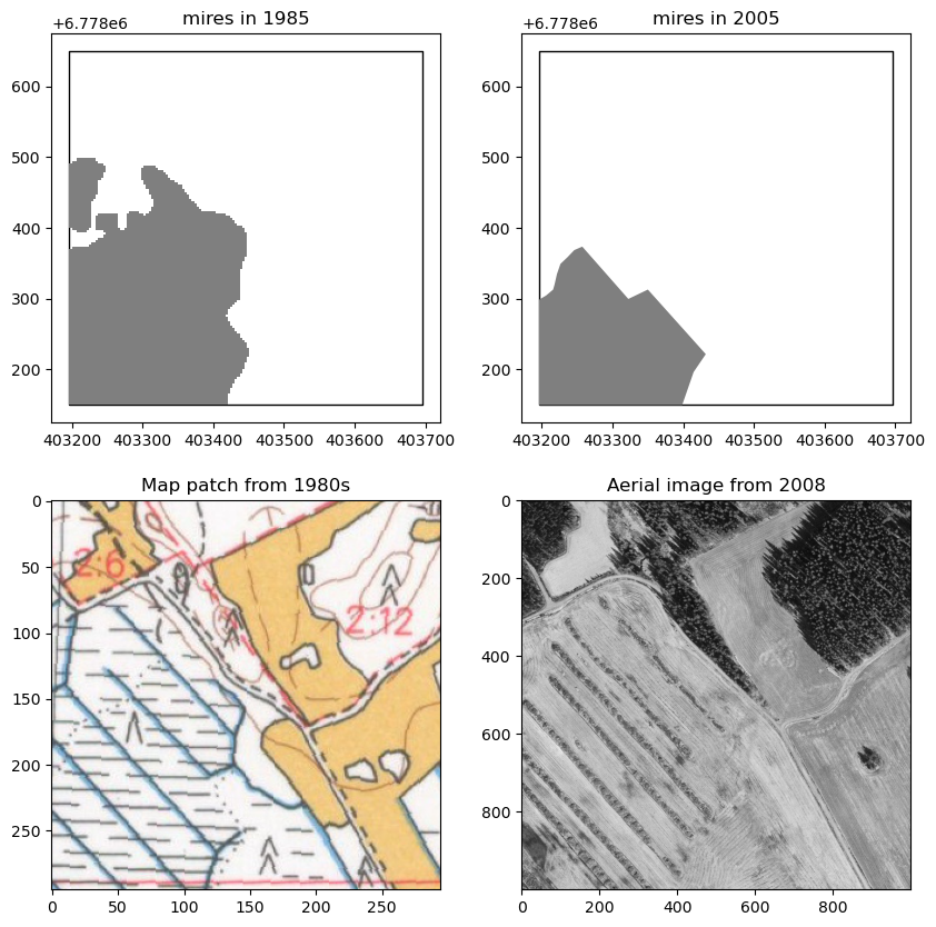
Same for 1985 and 2005
Code
= grid[grid.mire_change_8505 == grid.mire_change_8505.min ()].cellid.iloc[0 ]= plt.subplots(2 ,2 , figsize= (10 ,10 ))== mireloss_8505_cellid].plot(ax= axs[0 ,0 ], facecolor= 'none' )== mireloss_8505_cellid].geometry).plot(ax= axs[0 ,0 ], color= 'tab:gray' ).set_title('mires in 1985' )== mireloss_8505_cellid].plot(ax= axs[0 ,1 ], facecolor= 'none' )== mireloss_8505_cellid].geometry).plot(ax= axs[0 ,1 ], color= 'tab:gray' ).set_title('mires in 2005' )= get_map_patch(grid[grid.cellid == mireloss_8505_cellid].geometry.iloc[0 ], 1985 , map_path)1 ,0 ].imshow(img, cmap= 'gray' )1 ,0 ].set_title(f'Map patch from 1980s' )= get_wcs_img(grid[grid.cellid == mireloss_8505_cellid].total_bounds, 2005 )1 ,1 ].imshow(img, cmap= 'gray' )1 ,1 ].set_title(f'Aerial image from { year} ' )
Text(0.5, 1.0, 'Aerial image from 2008')
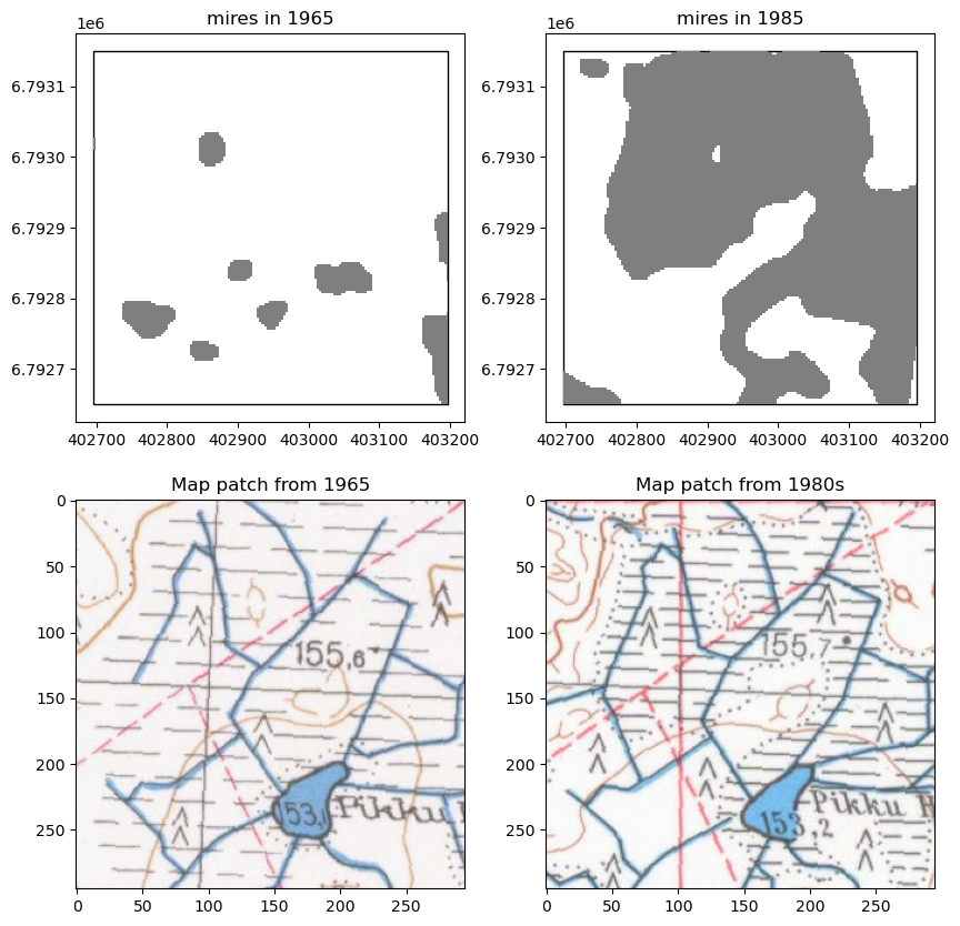
And then same visualizations for mire area increase.
Code
= grid[grid.mire_change_6585 == grid.mire_change_6585.max ()].cellid.iloc[0 ]= plt.subplots(2 ,2 , figsize= (10 ,10 ))== miregain_6585_cellid].plot(ax= axs[0 ,0 ], facecolor= 'none' )== miregain_6585_cellid].geometry).plot(ax= axs[0 ,0 ], color= 'tab:gray' ).set_title('mires in 1965' )== miregain_6585_cellid].plot(ax= axs[0 ,1 ], facecolor= 'none' )== miregain_6585_cellid].geometry).plot(ax= axs[0 ,1 ], color= 'tab:gray' ).set_title('mires in 1985' )= get_map_patch(grid[grid.cellid == miregain_6585_cellid].geometry.iloc[0 ], 1965 , map_path)1 ,0 ].imshow(img, cmap= 'gray' )1 ,0 ].set_title(f'Map patch from 1965' )= get_map_patch(grid[grid.cellid == miregain_6585_cellid].geometry.iloc[0 ], 1985 , map_path)1 ,1 ].imshow(img, cmap= 'gray' )1 ,1 ].set_title(f'Map patch from 1980s' )
Text(0.5, 1.0, 'Map patch from 1980s')
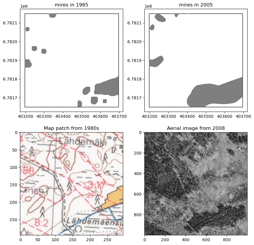
Code
= grid[grid.mire_change_8505 == grid.mire_change_8505.max ()].cellid.iloc[0 ]= plt.subplots(2 ,2 , figsize= (10 ,10 ))== miregain_8505_cellid].plot(ax= axs[0 ,0 ], facecolor= 'none' )== miregain_8505_cellid].geometry).plot(ax= axs[0 ,0 ], color= 'tab:gray' ).set_title('mires in 1985' )== miregain_8505_cellid].plot(ax= axs[0 ,1 ], facecolor= 'none' )== miregain_8505_cellid].geometry).plot(ax= axs[0 ,1 ], color= 'tab:gray' ).set_title('mires in 2005' )= get_map_patch(grid[grid.cellid == miregain_8505_cellid].geometry.iloc[0 ], 1985 , map_path)1 ,0 ].imshow(img, cmap= 'gray' )1 ,0 ].set_title(f'Map patch from 1980s' )= get_wcs_img(grid[grid.cellid == miregain_8505_cellid].total_bounds, 2005 )1 ,1 ].imshow(img, cmap= 'gray' )1 ,1 ].set_title(f'Aerial image from { year} ' )
Text(0.5, 1.0, 'Aerial image from 2008')
Roads
Code
= Path('../results/lines/roads/' )= None = None for p in os.listdir(road_path):= gpd.read_file(road_path/ p)if '1965' in p:if roads_65 is None : roads_65 = union_gdfelse : roads_65 = pd.concat((roads_65, union_gdf))else :if roads_80s is None : roads_80s = union_gdfelse : roads_80s = pd.concat((roads_80s, union_gdf))= roads_65[roads_65.geometry.length > 100 ]= roads_80s[roads_80s.geometry.length > 100 ] = roads_65.clip(study_area.geometry.iloc[0 ])= roads_80s.clip(study_area.geometry.iloc[0 ])= True , inplace= True )= True , inplace= True )= gpd.read_file(mtk_path/ '2005/roads.geojson' )= gpd.read_file(mtk_path/ '2022/tiet_2022.geojson' )= roads_22[roads_22.kohdeluokka.isin([12111 ,12112 ,12121 ,12122 ,12131 ,12132 ])]
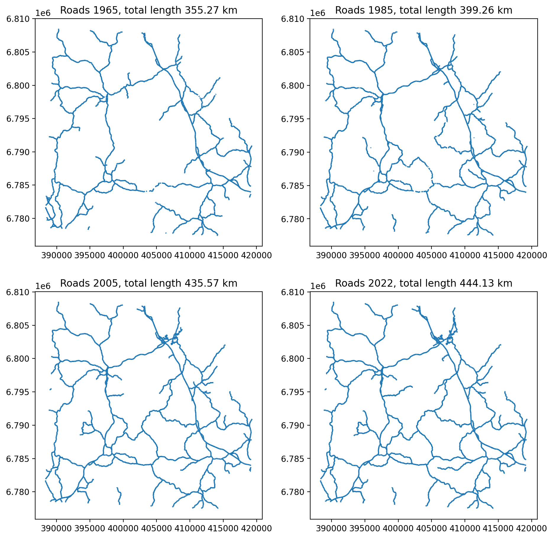
For roads, we can see the overall change in the road networks and approximate total length.
Code
= plt.subplots(2 ,2 , dpi= 200 , figsize= (11 ,11 ))= axs[0 ,0 ])= axs[0 ,1 ])= axs[1 ,0 ])= axs[1 ,1 ])0 ,0 ].set_title(f'Roads 1965, total length { roads_65. length. sum () * 10 **- 3 :.2f} km' )0 ,1 ].set_title(f'Roads 1985, total length { roads_80s. length. sum () * 10 **- 3 :.2f} km' )1 ,0 ].set_title(f'Roads 2005, total length { roads_05. length. sum () * 10 **- 3 :.2f} km' )1 ,1 ].set_title(f'Roads 2022, total length { roads_22. length. sum () * 10 **- 3 :.2f} km' )
Code
def get_len(cell, targs, sindex):= list (sindex.nearest(cell.geometry.bounds))= targs.iloc[nearest_idx]return tempdata.clip(cell.geometry, keep_geom_type= True ).length.sum () * 10 **- 3
Code
'road_length_65' ] = grid.progress_apply(lambda cell: get_len(cell, roads_65, roads_65.sindex), axis= 1 )'road_length_85' ] = grid.progress_apply(lambda cell: get_len(cell, roads_80s, roads_80s.sindex), axis= 1 )'road_length_05' ] = grid.progress_apply(lambda cell: get_len(cell, roads_05, roads_05.sindex), axis= 1 )'road_length_22' ] = grid.progress_apply(lambda cell: get_len(cell, roads_22, roads_22.sindex), axis= 1 )
100%|████████████████████████████████████████████████████████████████████████████| 4032/4032 [00:19<00:00, 211.94it/s]
100%|████████████████████████████████████████████████████████████████████████████| 4032/4032 [00:19<00:00, 203.38it/s]
100%|████████████████████████████████████████████████████████████████████████████| 4032/4032 [00:16<00:00, 249.25it/s]
100%|████████████████████████████████████████████████████████████████████████████| 4032/4032 [00:16<00:00, 244.59it/s]
Code
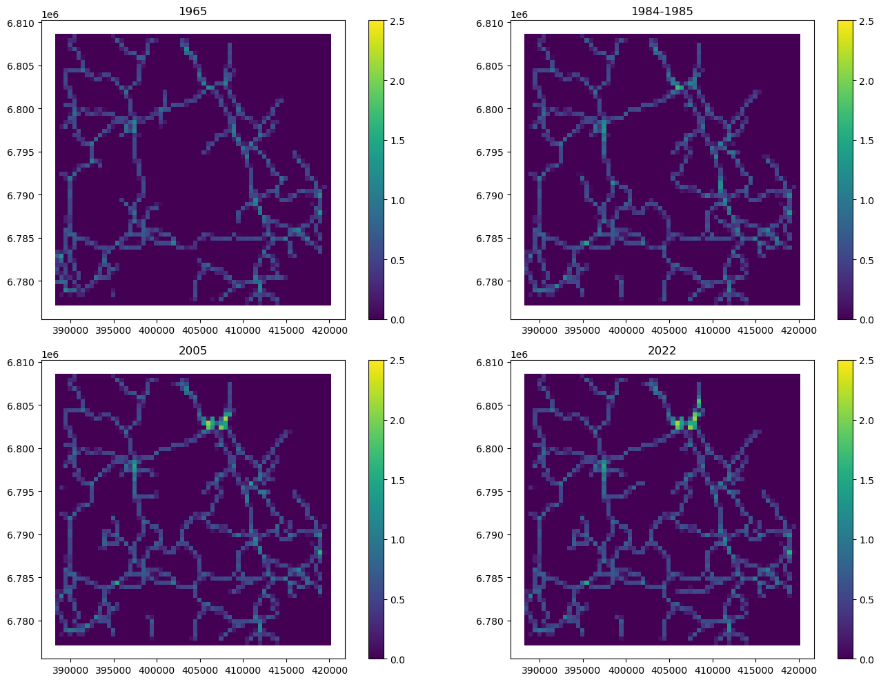
= plt.subplots(2 ,2 , figsize= (14 ,10 ))0 , inplace= True )= 'road_length_65' , ax= axs[0 ,0 ], vmin= 0 , vmax= 2.5 , legend= True ).set_title('1965' )= 'road_length_85' , ax= axs[0 ,1 ], vmin= 0 , vmax= 2.5 , legend= True ).set_title('1984-1985' )= 'road_length_05' , ax= axs[1 ,0 ], vmin= 0 , vmax= 2.5 , legend= True ).set_title('2005' )= 'road_length_22' , ax= axs[1 ,1 ], vmin= 0 , vmax= 2.5 , legend= True ).set_title('2022' )
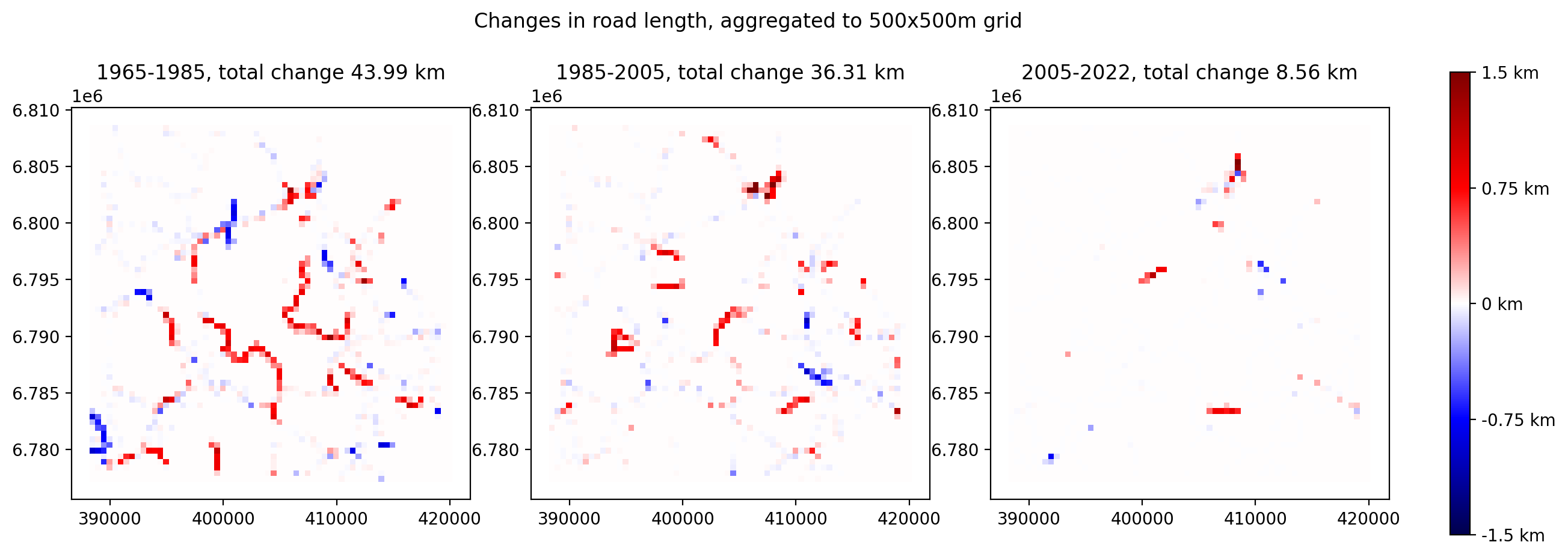
Quantify the change. Negative change means decreased road length.
Code
'road_change_6585' ] = (grid.road_length_85 - grid.road_length_65)'road_change_8505' ] = (grid.road_length_05 - grid.road_length_85)'road_change_0522' ] = (grid.road_length_22 - grid.road_length_05)
Change stats for 1965-1985:
Code
print (f'Gain: { grid[grid.road_change_6585 > 0 ]. road_change_6585. sum ():.2f} km' )print (f'Loss: { - grid[grid.road_change_6585 < 0 ]. road_change_6585. sum ():.2f} km' )print (f'Change: { grid. road_change_6585. sum ():.2f} km' )
Gain: 72.54 km
Loss: 28.55 km
Change: 43.99 km
Change stats for 1985-2005
Code
print (f'Gain: { grid[grid.road_change_8505 > 0 ]. road_change_8505. sum ():.2f} km' )print (f'Loss: { - grid[grid.road_change_8505 < 0 ]. road_change_8505. sum ():.2f} km' )print (f'Change: { grid. road_change_8505. sum ():.2f} km' )
Gain: 49.61 km
Loss: 13.30 km
Change: 36.31 km
Change stats for 2005-2022
Code
print (f'Gain: { grid[grid.road_change_0522 > 0 ]. road_change_0522. sum ():.2f} km' )print (f'Loss: { - grid[grid.road_change_0522 < 0 ]. road_change_0522. sum ():.2f} km' )print (f'Change: { grid. road_change_0522. sum ():.2f} km' )
Gain: 12.79 km
Loss: 4.24 km
Change: 8.56 km
Code
= plt.subplots(1 ,4 , figsize= (15 ,5 ), dpi= 200 , gridspec_kw= {'width_ratios' : [1 ,1 ,1 ,0.05 ]})= 'road_change_6585' , cmap= 'seismic' , vmin=- 1 , vmax= 1 , ax= axs[0 ])= 'road_change_8505' , cmap= 'seismic' , vmin=- 1 , vmax= 1 , ax= axs[1 ])= 'road_change_0522' , cmap= 'seismic' , vmin=- 1 , vmax= 1 , ax= axs[2 ])0 ].set_title(f'1965-1985, total change { grid. road_change_6585. sum ():.2f} km' )1 ].set_title(f'1985-2005, total change { grid. road_change_8505. sum ():.2f} km' )2 ].set_title(f'2005-2022, total change { grid. road_change_0522. sum ():.2f} km' )= colors.Normalize(vmin=- 1.5 ,vmax= 1.5 )= plt.cm.ScalarMappable(cmap= 'seismic' , norm= norm)= [- 1.5 ,- 0.75 ,0 ,0.75 ,1.5 ]= plt.colorbar(sm, cax= axs[3 ], ticks= ticks)f' { t} km' for t in ticks])'Changes in road length, aggregated to 500x500m grid' )
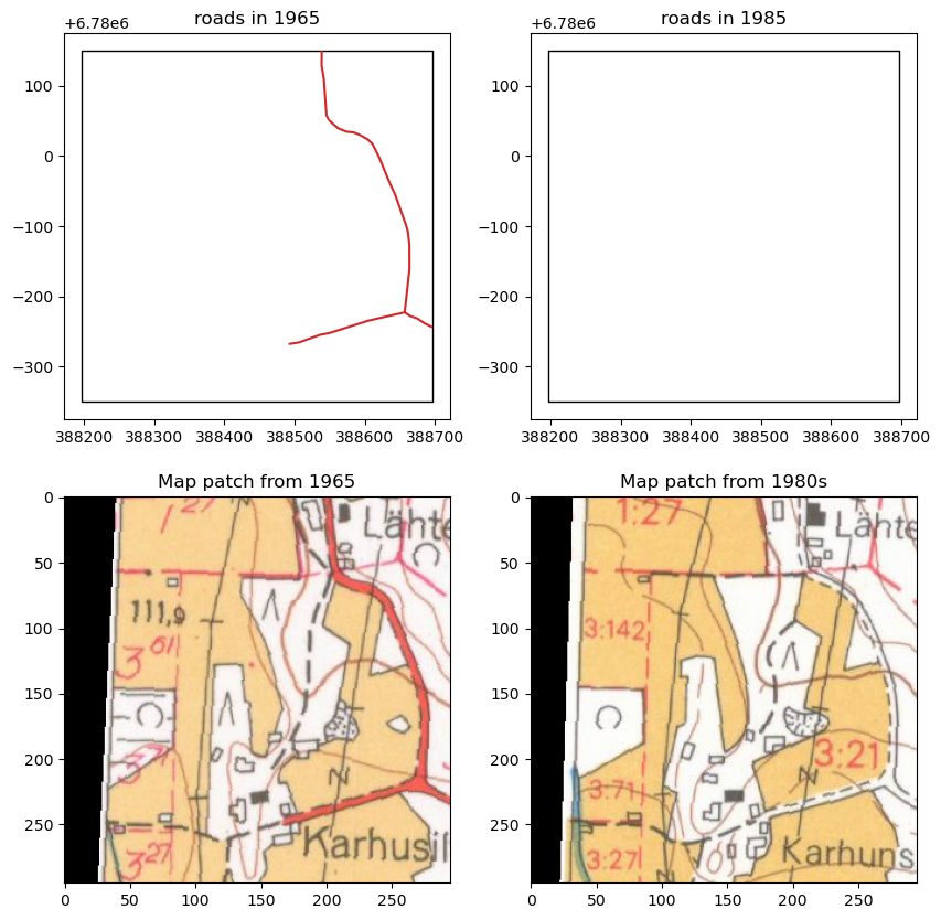
Visualize the location where the road length has decreased the most between 1965 and 1985. For 1965 and 1980s show the corresponding map patch along with the data.
For 2005 and 2022, show the closest aerial image to that year. Unfortunately the closest historical images available are from 1949 and 1979, so we can’t really use them for visualizations.
Code
= Path('../data/maps/aligned_maps/' )= grid[grid.road_change_6585 == grid.road_change_6585.min ()].cellid.iloc[0 ]= plt.subplots(2 ,2 , figsize= (10 ,10 ))== roadloss_6585_cellid].plot(ax= axs[0 ,0 ], facecolor= 'none' )== roadloss_6585_cellid].geometry).plot(ax= axs[0 ,0 ], color= 'tab:red' ).set_title('roads in 1965' )== roadloss_6585_cellid].plot(ax= axs[0 ,1 ], facecolor= 'none' )== roadloss_6585_cellid].geometry).plot(ax= axs[0 ,1 ], color= 'tab:red' ).set_title('roads in 1985' )= get_map_patch(grid[grid.cellid == roadloss_6585_cellid].geometry.iloc[0 ], 1965 , map_path)1 ,0 ].imshow(img, cmap= 'gray' )1 ,0 ].set_title(f'Map patch from 1965' )= get_map_patch(grid[grid.cellid == roadloss_6585_cellid].geometry.iloc[0 ], 1985 , map_path)1 ,1 ].imshow(img, cmap= 'gray' )1 ,1 ].set_title(f'Map patch from 1980s' )
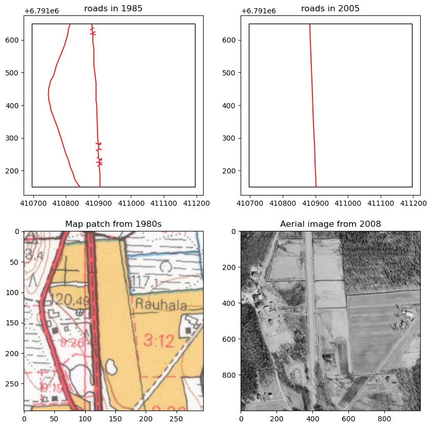
Same for 1985 and 2005
Code
= grid[grid.road_change_8505 == grid.road_change_8505.min ()].cellid.iloc[0 ]= plt.subplots(2 ,2 , figsize= (10 ,10 ))== roadloss_8505_cellid].plot(ax= axs[0 ,0 ], facecolor= 'none' )== roadloss_8505_cellid].geometry).plot(ax= axs[0 ,0 ], color= 'tab:red' ).set_title('roads in 1985' )== roadloss_8505_cellid].plot(ax= axs[0 ,1 ], facecolor= 'none' )== roadloss_8505_cellid].geometry).plot(ax= axs[0 ,1 ], color= 'tab:red' ).set_title('roads in 2005' )= get_map_patch(grid[grid.cellid == roadloss_8505_cellid].geometry.iloc[0 ], 1985 , map_path)1 ,0 ].imshow(img, cmap= 'gray' )1 ,0 ].set_title(f'Map patch from 1980s' )= get_wcs_img(grid[grid.cellid == roadloss_8505_cellid].total_bounds, 2005 )1 ,1 ].imshow(img, cmap= 'gray' )1 ,1 ].set_title(f'Aerial image from { year} ' )
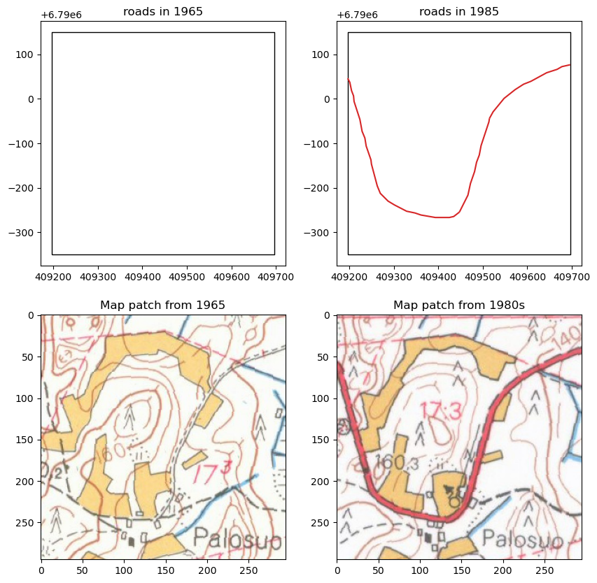
And then same visualizations for road length increase.
Code
= grid[grid.road_change_6585 == grid.road_change_6585.max ()].cellid.iloc[0 ]= plt.subplots(2 ,2 , figsize= (10 ,10 ))== roadgain_6585_cellid].plot(ax= axs[0 ,0 ], facecolor= 'none' )== roadgain_6585_cellid].geometry).plot(ax= axs[0 ,0 ], color= 'tab:red' ).set_title('roads in 1965' )== roadgain_6585_cellid].plot(ax= axs[0 ,1 ], facecolor= 'none' )== roadgain_6585_cellid].geometry).plot(ax= axs[0 ,1 ], color= 'tab:red' ).set_title('roads in 1985' )= get_map_patch(grid[grid.cellid == roadgain_6585_cellid].geometry.iloc[0 ], 1965 , map_path)1 ,0 ].imshow(img, cmap= 'gray' )1 ,0 ].set_title(f'Map patch from 1965' )= get_map_patch(grid[grid.cellid == roadgain_6585_cellid].geometry.iloc[0 ], 1985 , map_path)1 ,1 ].imshow(img, cmap= 'gray' )1 ,1 ].set_title(f'Map patch from 1980s' )
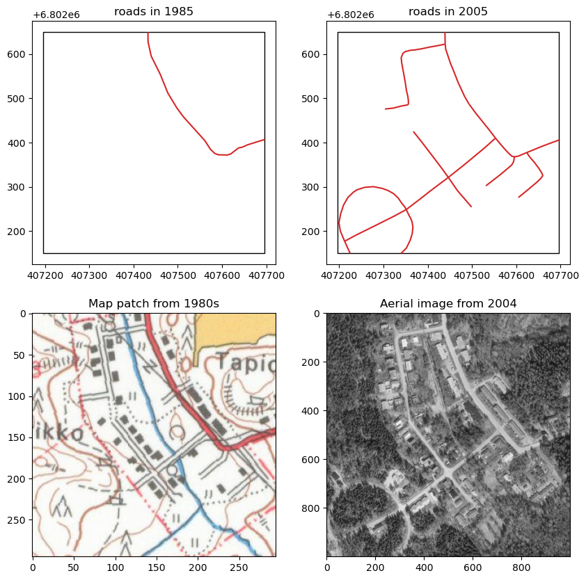
Code
= grid[grid.road_change_8505 == grid.road_change_8505.max ()].cellid.iloc[0 ]= plt.subplots(2 ,2 , figsize= (10 ,10 ))== roadgain_8505_cellid].plot(ax= axs[0 ,0 ], facecolor= 'none' )== roadgain_8505_cellid].geometry).plot(ax= axs[0 ,0 ], color= 'tab:red' ).set_title('roads in 1985' )== roadgain_8505_cellid].plot(ax= axs[0 ,1 ], facecolor= 'none' )== roadgain_8505_cellid].geometry).plot(ax= axs[0 ,1 ], color= 'tab:red' ).set_title('roads in 2005' )= get_map_patch(grid[grid.cellid == roadgain_8505_cellid].geometry.iloc[0 ], 1985 , map_path)1 ,0 ].imshow(img, cmap= 'gray' )1 ,0 ].set_title(f'Map patch from 1980s' )= get_wcs_img(grid[grid.cellid == roadgain_8505_cellid].total_bounds, 2005 )1 ,1 ].imshow(img, cmap= 'gray' )1 ,1 ].set_title(f'Aerial image from { year} ' )
Watercourses
Code
= Path('../results/lines/watercourses/' )= None = None for p in os.listdir(ww_path):= gpd.read_file(ww_path/ p)if '1965' in p:if watercourses_65 is None : watercourses_65 = union_gdfelse : watercourses_65 = pd.concat((watercourses_65, union_gdf))else :if watercourses_80s is None : watercourses_80s = union_gdfelse : watercourses_80s = pd.concat((watercourses_80s, union_gdf))= mires_65.clip(study_area.geometry.iloc[0 ])= mires_80s.clip(study_area.geometry.iloc[0 ])= True , inplace= True )= True , inplace= True )= gpd.read_file(mtk_path/ '2005/watercourses.geojson' )= gpd.read_file(mtk_path/ '2022/virtavedet_2022.geojson' )
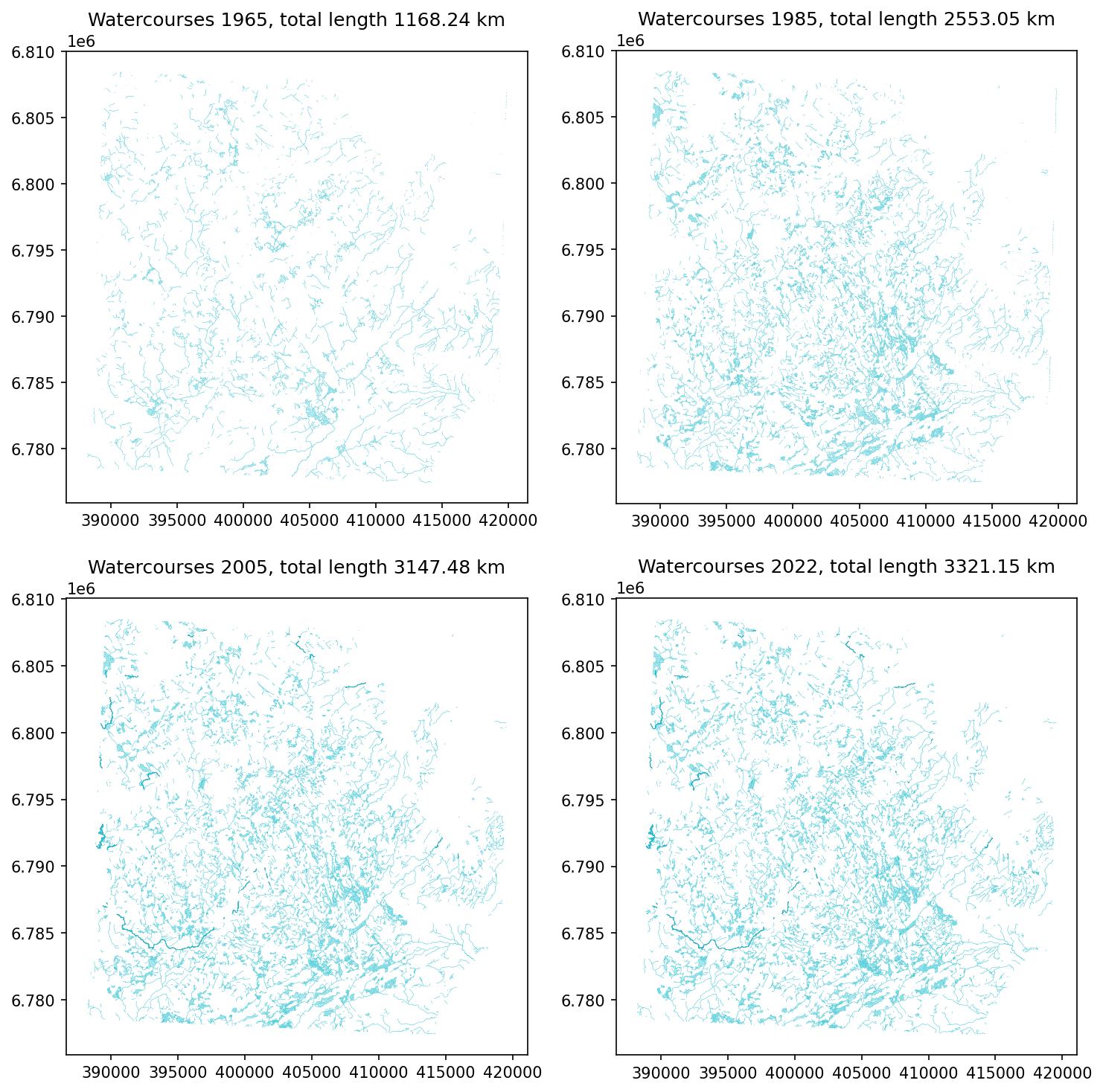
Code
= plt.subplots(2 ,2 , figsize= (10 ,10 ), dpi= 150 )= axs[0 ,0 ], color= 'tab:cyan' , linewidth= .2 )0 ,0 ].set_title(f'Watercourses 1965, total length { (watercourses_65.length.sum () * 10 **- 3 ):.2f} km' )= axs[0 ,1 ], color= 'tab:cyan' , linewidth= .2 )0 ,1 ].set_title(f'Watercourses 1985, total length { (watercourses_80s.length.sum () * 10 **- 3 ):.2f} km' )= axs[1 ,0 ], color= 'tab:cyan' , linewidth= .2 )1 ,0 ].set_title(f'Watercourses 2005, total length { (watercourses_05.length.sum () * 10 **- 3 ):.2f} km' )= axs[1 ,1 ], color= 'tab:cyan' , linewidth= .2 )1 ,1 ].set_title(f'Watercourses 2022, total length { (watercourses_22.length.sum () * 10 **- 3 ):.2f} km' )
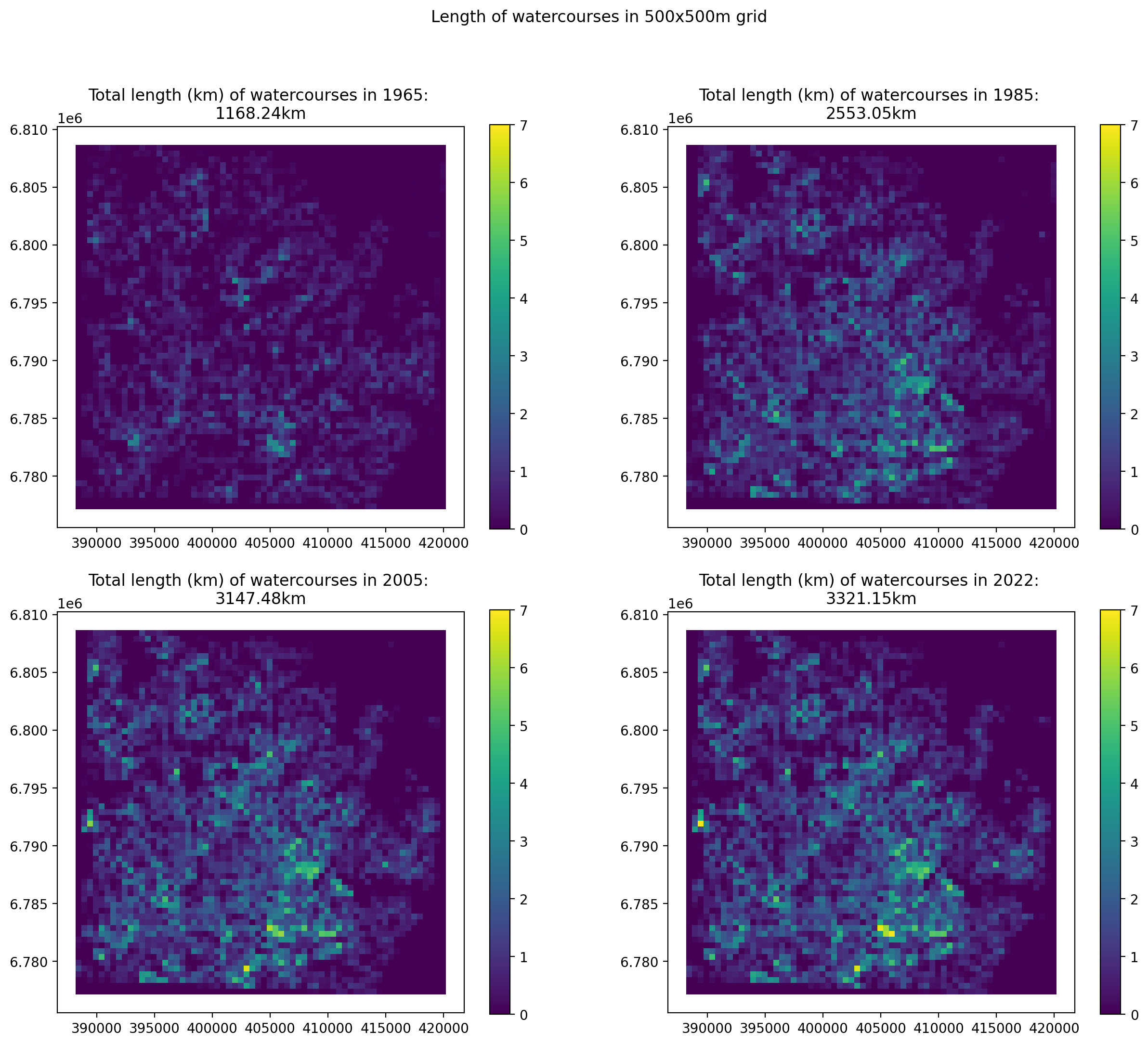
Again, to make finding the ditching hotspots easier, aggregate the data into 500x500m grid.
Code
'watercourse_length_65' ] = grid.progress_apply(lambda cell: get_len(cell, watercourses_65, watercourses_65.sindex), axis= 1 )'watercourse_length_85' ] = grid.progress_apply(lambda cell: get_len(cell, watercourses_80s, watercourses_80s.sindex), axis= 1 )'watercourse_length_05' ] = grid.progress_apply(lambda cell: get_len(cell, watercourses_05, watercourses_05.sindex), axis= 1 )'watercourse_length_22' ] = grid.progress_apply(lambda cell: get_len(cell, watercourses_22, watercourses_22.sindex), axis= 1 )
Code
= plt.subplots(2 ,2 , figsize= (15 ,12 ), dpi= 200 )= 'watercourse_length_65' , ax= axs[0 ,0 ], vmin= 0 , vmax= 7 , legend= True )0 ,0 ].set_title(f'Total length (km) of watercourses in 1965: \n { grid. watercourse_length_65. sum () :.2f} km' )= 'watercourse_length_85' , ax= axs[0 ,1 ], vmin= 0 , vmax= 7 , legend= True )0 ,1 ].set_title(f'Total length (km) of watercourses in 1985: \n { grid. watercourse_length_85. sum () :.2f} km' )= 'watercourse_length_05' , ax= axs[1 ,0 ], vmin= 0 , vmax= 7 , legend= True )1 ,0 ].set_title(f'Total length (km) of watercourses in 2005: \n { grid. watercourse_length_05. sum () :.2f} km' )= 'watercourse_length_22' , ax= axs[1 ,1 ], vmin= 0 , vmax= 7 , legend= True )1 ,1 ].set_title(f'Total length (km) of watercourses in 2022: \n { grid. watercourse_length_22. sum () :.2f} km' )'Length of watercourses in 500x500m grid' )
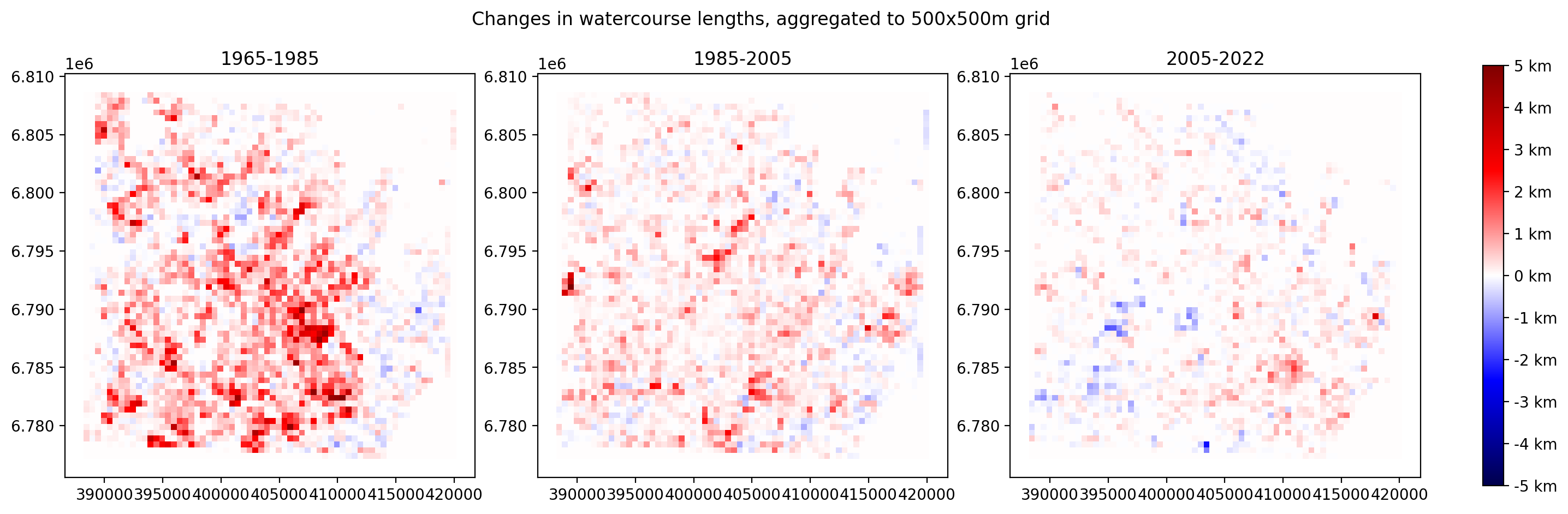
Then visualize the changes between the years.
Code
'watercourse_change_6585' ] = (grid.watercourse_length_85 - grid.watercourse_length_65) 'watercourse_change_8505' ] = (grid.watercourse_length_05 - grid.watercourse_length_85) 'watercourse_change_0522' ] = (grid.watercourse_length_22 - grid.watercourse_length_05)
Change stats for 1965-1985:
Code
print (f'Gain: { grid[grid.watercourse_change_6585 > 0 ]. watercourse_change_6585. sum ():.2f} km' )print (f'Loss: { - grid[grid.watercourse_change_6585 < 0 ]. watercourse_change_6585. sum ():.2f} km' )print (f'Change: { grid. watercourse_change_6585. sum ():.2f} km' )
Gain: 1473.98 km
Loss: 89.17 km
Change: 1384.81 km
Change stats for 1985-2005
Code
print (f'Gain: { grid[grid.watercourse_change_8505 > 0 ]. watercourse_change_8505. sum ():.2f} km' )print (f'Loss: { - grid[grid.watercourse_change_8505 < 0 ]. watercourse_change_8505. sum ():.2f} km' )print (f'Change: { grid. watercourse_change_8505. sum ():.2f} km' )
Gain: 689.11 km
Loss: 94.68 km
Change: 594.43 km
Change stats for 2005-2022
Code
print (f'Gain: { grid[grid.watercourse_change_0522 > 0 ]. watercourse_change_0522. sum ():.2f} km' )print (f'Loss: { - grid[grid.watercourse_change_0522 < 0 ]. watercourse_change_0522. sum ():.2f} km' )print (f'Change: { grid. watercourse_change_0522. sum ():.2f} km' )
Gain: 281.52 km
Loss: 107.85 km
Change: 173.67 km
Code
import matplotlib.colors as colors= plt.subplots(1 ,4 , figsize= (17 ,5 ), dpi= 200 , gridspec_kw= {'width_ratios' : [1 ,1 ,1 ,0.05 ]})= 'watercourse_change_6585' , ax= axs[0 ], vmin=- 5 , vmax= 5 , cmap= 'seismic' )= 'watercourse_change_8505' , ax= axs[1 ], vmin=- 5 , vmax= 5 , cmap= 'seismic' )= 'watercourse_change_0522' , ax= axs[2 ], vmin=- 5 , vmax= 5 , cmap= 'seismic' )0 ].set_title('1965-1985' )1 ].set_title('1985-2005' )2 ].set_title('2005-2022' )= colors.Normalize(vmin=- 5 ,vmax= 5 )= plt.cm.ScalarMappable(cmap= 'seismic' , norm= norm)= [- 5 ,- 4 ,- 3 ,- 2 ,- 1 ,0 ,1 ,2 ,3 ,4 ,5 ]= plt.colorbar(sm, cax= axs[3 ], ticks= ticks)f' { t} km' for t in ticks])'Changes in watercourse lengths, aggregated to 500x500m grid' )
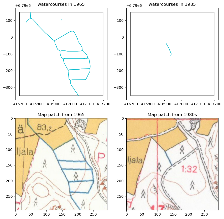
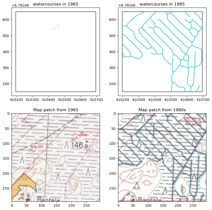
Visualize the locations where there has been the most decrease in watercourse length between 1965 and 1985.
Code
= grid[grid.watercourse_change_6585 == grid.watercourse_change_6585.min ()].cellid.iloc[0 ]= plt.subplots(2 ,2 , figsize= (10 ,10 ))== watercourseloss_6585_cellid].plot(ax= axs[0 ,0 ], facecolor= 'none' )== watercourseloss_6585_cellid].geometry).plot(ax= axs[0 ,0 ], color= 'tab:cyan' ).set_title('watercourses in 1965' )== watercourseloss_6585_cellid].plot(ax= axs[0 ,1 ], facecolor= 'none' )== watercourseloss_6585_cellid].geometry).plot(ax= axs[0 ,1 ], color= 'tab:cyan' ).set_title('watercourses in 1985' )= get_map_patch(grid[grid.cellid == watercourseloss_6585_cellid].geometry.iloc[0 ], 1965 , map_path)1 ,0 ].imshow(img, cmap= 'gray' )1 ,0 ].set_title(f'Map patch from 1965' )= get_map_patch(grid[grid.cellid == watercourseloss_6585_cellid].geometry.iloc[0 ], 1985 , map_path)1 ,1 ].imshow(img, cmap= 'gray' )1 ,1 ].set_title(f'Map patch from 1980s' )
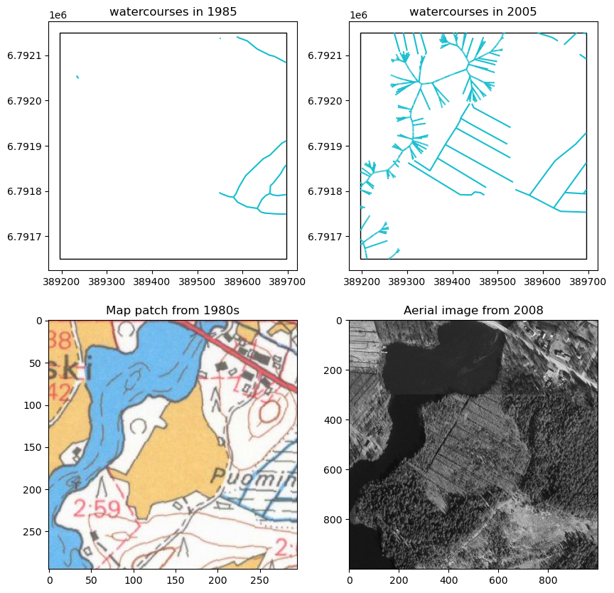
Same for 1985 and 2005
Code
= grid[grid.watercourse_change_8505 == grid.watercourse_change_8505.min ()].cellid.iloc[0 ]= plt.subplots(2 ,2 , figsize= (10 ,10 ))== watercourseloss_8505_cellid].plot(ax= axs[0 ,0 ], facecolor= 'none' )== watercourseloss_8505_cellid].geometry).plot(ax= axs[0 ,0 ], color= 'tab:cyan' ).set_title('watercourses in 1985' )== watercourseloss_8505_cellid].plot(ax= axs[0 ,1 ], facecolor= 'none' )== watercourseloss_8505_cellid].geometry).plot(ax= axs[0 ,1 ], color= 'tab:cyan' ).set_title('watercourses in 2005' )= get_map_patch(grid[grid.cellid == watercourseloss_8505_cellid].geometry.iloc[0 ], 1985 , map_path)1 ,0 ].imshow(img, cmap= 'gray' )1 ,0 ].set_title(f'Map patch from 1980s' )= get_wcs_img(grid[grid.cellid == watercourseloss_8505_cellid].total_bounds, 2005 )1 ,1 ].imshow(img, cmap= 'gray' )1 ,1 ].set_title(f'Aerial image from { year} ' )
And then same visualizations for watercourse length increase.
Code
= grid[grid.watercourse_change_6585 == grid.watercourse_change_6585.max ()].cellid.iloc[0 ]= plt.subplots(2 ,2 , figsize= (10 ,10 ))== watercoursegain_6585_cellid].plot(ax= axs[0 ,0 ], facecolor= 'none' )== watercoursegain_6585_cellid].geometry).plot(ax= axs[0 ,0 ], color= 'tab:cyan' ).set_title('watercourses in 1965' )== watercoursegain_6585_cellid].plot(ax= axs[0 ,1 ], facecolor= 'none' )== watercoursegain_6585_cellid].geometry).plot(ax= axs[0 ,1 ], color= 'tab:cyan' ).set_title('watercourses in 1985' )= get_map_patch(grid[grid.cellid == watercoursegain_6585_cellid].geometry.iloc[0 ], 1965 , map_path)1 ,0 ].imshow(img, cmap= 'gray' )1 ,0 ].set_title(f'Map patch from 1965' )= get_map_patch(grid[grid.cellid == watercoursegain_6585_cellid].geometry.iloc[0 ], 1985 , map_path)1 ,1 ].imshow(img, cmap= 'gray' )1 ,1 ].set_title(f'Map patch from 1980s' )
Code
= grid[grid.watercourse_change_8505 == grid.watercourse_change_8505.max ()].cellid.iloc[0 ]= plt.subplots(2 ,2 , figsize= (10 ,10 ))== watercoursegain_8505_cellid].plot(ax= axs[0 ,0 ], facecolor= 'none' )== watercoursegain_8505_cellid].geometry).plot(ax= axs[0 ,0 ], color= 'tab:cyan' ).set_title('watercourses in 1985' )== watercoursegain_8505_cellid].plot(ax= axs[0 ,1 ], facecolor= 'none' )== watercoursegain_8505_cellid].geometry).plot(ax= axs[0 ,1 ], color= 'tab:cyan' ).set_title('watercourses in 2005' )= get_map_patch(grid[grid.cellid == watercoursegain_8505_cellid].geometry.iloc[0 ], 1985 , map_path)1 ,0 ].imshow(img, cmap= 'gray' )1 ,0 ].set_title(f'Map patch from 1980s' )= get_wcs_img(grid[grid.cellid == watercoursegain_8505_cellid].total_bounds, 2005 )1 ,1 ].imshow(img, cmap= 'gray' )1 ,1 ].set_title(f'Aerial image from { year} ' )
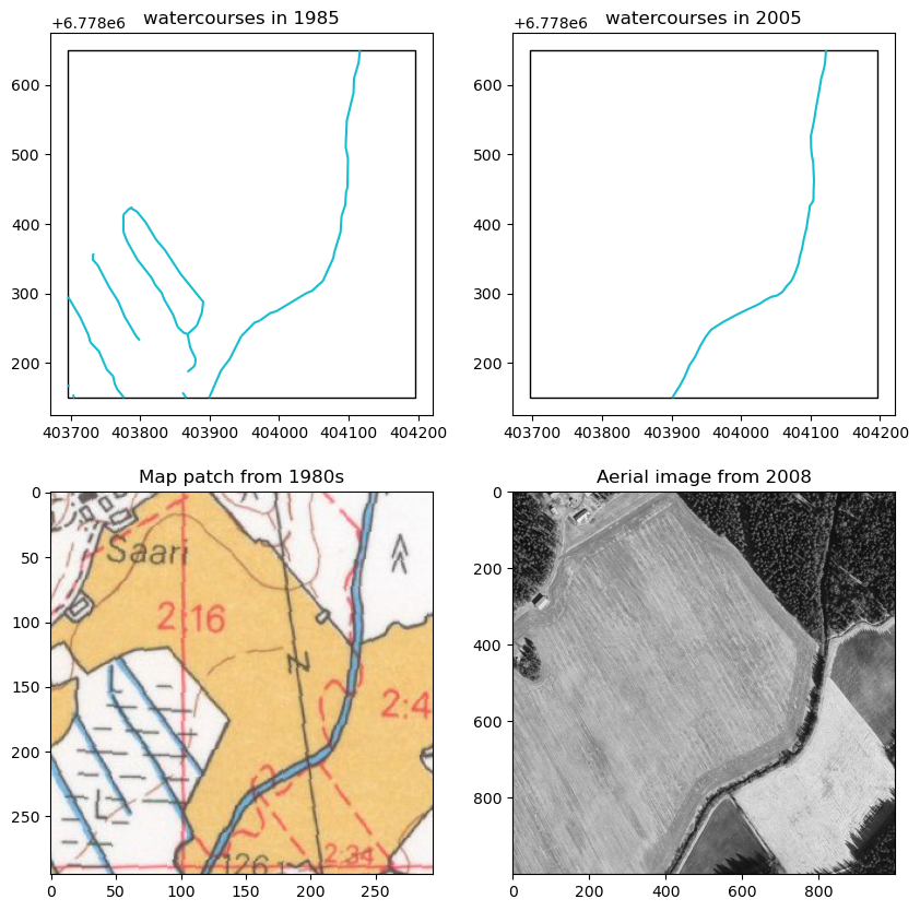
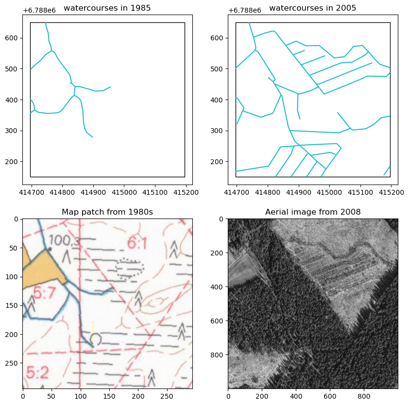
The example above shows the difficulty of distinguishing between water bodies and watercourses, and how converting some watercourses into line geometries may fail. See a better example with the fifth highest.
Code
= grid[grid.watercourse_change_8505 == np.partition(grid.watercourse_change_8505.values, - 5 )[- 5 ]].cellid.iloc[0 ]= plt.subplots(2 ,2 , figsize= (10 ,10 ))== watercoursegain_8505_cellid].plot(ax= axs[0 ,0 ], facecolor= 'none' )== watercoursegain_8505_cellid].geometry).plot(ax= axs[0 ,0 ], color= 'tab:cyan' ).set_title('watercourses in 1985' )== watercoursegain_8505_cellid].plot(ax= axs[0 ,1 ], facecolor= 'none' )== watercoursegain_8505_cellid].geometry).plot(ax= axs[0 ,1 ], color= 'tab:cyan' ).set_title('watercourses in 2005' )= get_map_patch(grid[grid.cellid == watercoursegain_8505_cellid].geometry.iloc[0 ], 1985 , map_path)1 ,0 ].imshow(img, cmap= 'gray' )1 ,0 ].set_title(f'Map patch from 1980s' )= get_wcs_img(grid[grid.cellid == watercoursegain_8505_cellid].total_bounds, 2005 )1 ,1 ].imshow(img, cmap= 'gray' )1 ,1 ].set_title(f'Aerial image from { year} ' )
Field-watercourse -combinations
Check how ditching has changed in fields, e.g. does shift to sub-surface drainage systems show in these data.
Code
'drainage_len' ] = fields_65.progress_apply(lambda row: get_len(row, watercourses_65, watercourses_65.sindex), axis= 1 )'drainage_len' ] = fields_80s.progress_apply(lambda row: get_len(row, watercourses_80s, watercourses_80s.sindex), axis= 1 )'drainage_len' ] = fields_05.progress_apply(lambda row: get_len(row, watercourses_05, watercourses_05.sindex), axis= 1 )'drainage_len' ] = fields_22.progress_apply(lambda row: get_len(row, watercourses_22, watercourses_22.sindex), axis= 1 )
Code
print (f'Total length of waterways in fields in 1965: { fields_65. drainage_len. sum ():.2f} km' ) print (f'Total length of waterways in fields in 1985: { fields_80s. drainage_len. sum ():.2f} km' ) print (f'Total length of waterways in fields in 2005: { fields_05. drainage_len. sum ():.2f} km' ) print (f'Total length of waterways in fields in 2022: { fields_22. drainage_len. sum ():.2f} km' )
Total length of waterways in fields in 1965: 266.62 km
Total length of waterways in fields in 1985: 273.78 km
Total length of waterways in fields in 2005: 194.06 km
Total length of waterways in fields in 2022: 166.73 km
Mire-watercourse -combinations
Code
'drainage_len' ] = mires_65.progress_apply(lambda row: get_len(row, watercourses_65, watercourses_65.sindex), axis= 1 )'drainage_len' ] = mires_80s.progress_apply(lambda row: get_len(row, watercourses_80s, watercourses_80s.sindex), axis= 1 )'drainage_len' ] = mires_05.progress_apply(lambda row: get_len(row, watercourses_05, watercourses_05.sindex), axis= 1 )'drainage_len' ] = mires_22.progress_apply(lambda row: get_len(row, watercourses_22, watercourses_22.sindex), axis= 1 )
Code
print (f'Total length of waterways in mires in 1965: { mires_65. drainage_len. sum ():.2f} km' ) print (f'Total length of waterways in mires in 1985: { mires_80s. drainage_len. sum ():.2f} km' ) print (f'Total length of waterways in mires in 2005: { mires_05. drainage_len. sum ():.2f} km' ) print (f'Total length of waterways in mires in 2022: { mires_22. drainage_len. sum ():.2f} km' )
Total length of waterways in mires in 1965: 447.12 km
Total length of waterways in mires in 1985: 1604.50 km
Total length of waterways in mires in 2005: 1925.36 km
Total length of waterways in mires in 2022: 2104.92 km
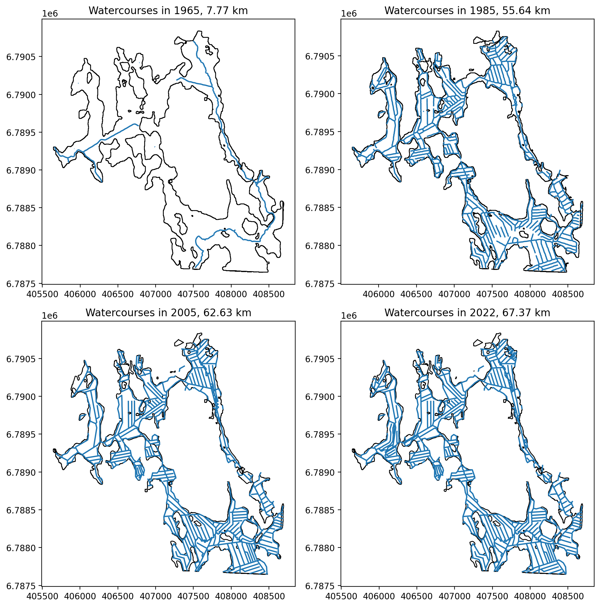
Watercourse changes can indicating ditching or restoration can be visualized for mires area. In this example, we use the mire layer from 1965 maps as the aggregation layer.
Code
'drainage_len_65' ] = mires_65.progress_apply(lambda row: get_len(row, watercourses_65, watercourses_65.sindex), axis= 1 )'drainage_len_85' ] = mires_65.progress_apply(lambda row: get_len(row, watercourses_80s, watercourses_80s.sindex), axis= 1 )'drainage_len_05' ] = mires_65.progress_apply(lambda row: get_len(row, watercourses_05, watercourses_05.sindex), axis= 1 )'drainage_len_22' ] = mires_65.progress_apply(lambda row: get_len(row, watercourses_22, watercourses_22.sindex), axis= 1 )
Code
'drain_change_6585' ] = (mires_65.drainage_len_85 - mires_65.drainage_len_65)'drain_change_8505' ] = (mires_65.drainage_len_05 - mires_65.drainage_len_85)'drain_change_0522' ] = (mires_65.drainage_len_22 - mires_65.drainage_len_05)
Filter out the mire where the ditching has been the most aggressive between 1965 and 1985.
Code
= mires_65[mires_65.drain_change_6585 == mires_65.drain_change_6585.max ()].geometry.iloc[0 ]= plt.subplots(2 ,2 , dpi= 200 , figsize= (10 ,10 ))= True ).plot(ax= axs[0 ,0 ], facecolor= 'none' )= True ).plot(ax= axs[0 ,1 ], facecolor= 'none' )= True ).plot(ax= axs[1 ,0 ], facecolor= 'none' )= True ).plot(ax= axs[1 ,1 ], facecolor= 'none' )= True ).plot(ax= axs[0 ,0 ])= axs[0 ,1 ])= axs[1 ,0 ])= axs[1 ,1 ])0 ,0 ].set_title(f'Watercourses in 1965, { watercourses_65. clip(largest_mire). length. sum ()* 10 **- 3 :.2f} km' )0 ,1 ].set_title(f'Watercourses in 1985, { watercourses_80s. clip(largest_mire). length. sum ()* 10 **- 3 :.2f} km' )1 ,0 ].set_title(f'Watercourses in 2005, { watercourses_05. clip(largest_mire). length. sum ()* 10 **- 3 :.2f} km' )1 ,1 ].set_title(f'Watercourses in 2022, { watercourses_22. clip(largest_mire). length. sum ()* 10 **- 3 :.2f} km' )
Same area as map patches and aerial images.
Code
= plt.subplots(2 ,2 , dpi= 200 , figsize= (10 ,10 ))= get_map_patch(box(* largest_mire.bounds), 1965 , map_path)for a in axs.flatten(): a.axis('off' )0 ,0 ].imshow(img, cmap= 'gray' )0 ,0 ].set_title(f'Map patch from 1965' )= get_map_patch(box(* largest_mire.bounds), 1985 , map_path)0 ,1 ].imshow(img, cmap= 'gray' )0 ,1 ].set_title(f'Map patch from 1980s' )# WCS only supports 2x2km images so need to get creative = (largest_mire.bounds[2 ] - largest_mire.bounds[0 ]) / 2 = (largest_mire.bounds[3 ] - largest_mire.bounds[1 ]) / 2 = get_wcs_img((largest_mire.bounds[0 ], 1 ], 2 ]- midx, 3 ]- midy), 2005 )= get_wcs_img((largest_mire.bounds[2 ]- midx, 1 ], 2 ], 3 ]- midy), 2005 )= get_wcs_img((largest_mire.bounds[0 ], 3 ]- midy, 2 ]- midx, 3 ]), 2005 )= get_wcs_img((largest_mire.bounds[2 ]- midx, 3 ]- midy, 2 ],3 ]), 2005 )= np.hstack((topl, topr))= np.hstack((botl, botr))= np.vstack((toprow, botrow))1 ,0 ].imshow(full, cmap= 'gray' )1 ,0 ].set_title(f'Aerial image from { year} ' )= get_wcs_img((largest_mire.bounds[0 ], 1 ], 2 ]- midx, 3 ]- midy), 2022 )= get_wcs_img((largest_mire.bounds[2 ]- midx, 1 ], 2 ], 3 ]- midy), 2022 )= get_wcs_img((largest_mire.bounds[0 ], 3 ]- midy, 2 ]- midx, 3 ]), 2022 )= get_wcs_img((largest_mire.bounds[2 ]- midx, 3 ]- midy, 2 ],3 ]), 2022 )= np.hstack((topl, topr))= np.hstack((botl, botr))= np.vstack((toprow, botrow))1 ,1 ].imshow(full, cmap= 'gray' )1 ,1 ].set_title(f'Aerial image from { year} ' )
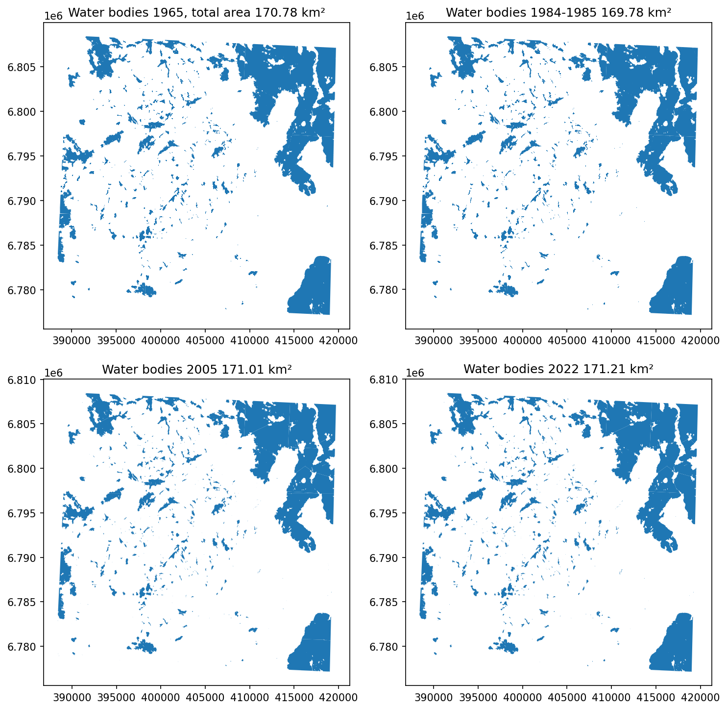
Water bodies
Even though water bodies don’t change that much, let’s visualize them for completeness.
Code
for r in results:/ r, polypath/ 'waterbodies' / r.replace('tif' , 'geojson' ), target_class= 5 , scale_factor= 1 / 2 )
Code
= None = None for p in os.listdir(polypath/ 'waterbodies' ):= gpd.read_file(polypath/ 'waterbodies' / p)if '1965' in p:if waterbodies_65 is None : waterbodies_65 = union_gdfelse : waterbodies_65 = pd.concat((waterbodies_65, union_gdf))else :if waterbodies_80s is None : waterbodies_80s = union_gdfelse : waterbodies_80s = pd.concat((waterbodies_80s, union_gdf))= waterbodies_65.clip(study_area.geometry.iloc[0 ])= waterbodies_80s.clip(study_area.geometry.iloc[0 ])= True , drop= True )= True , drop= True )= gpd.read_file(mtk_path/ '2005/waterbodies.geojson' )= gpd.read_file(mtk_path/ '2022/jarvet_2022.geojson' )
Code
= plt.subplots(2 ,2 , figsize= (10 ,10 ), dpi= 150 )= axs[0 ,0 ], color= 'tab:blue' )0 ,0 ].set_title(f'Water bodies 1965, total area { waterbodies_65. area. sum () * 10 **- 6 :.2f} km²' )= axs[0 ,1 ], color= 'tab:blue' )0 ,1 ].set_title(f'Water bodies 1984-1985 { waterbodies_80s. area. sum () * 10 **- 6 :.2f} km²' )= axs[1 ,0 ], color= 'tab:blue' )1 ,0 ].set_title(f'Water bodies 2005 { waterbodies_05. area. sum () * 10 **- 6 :.2f} km²' )= axs[1 ,1 ], color= 'tab:blue' )1 ,1 ].set_title(f'Water bodies 2022 { waterbodies_22. area. sum () * 10 **- 6 :.2f} km²' )
Some changes are due to model classifying wide rivers etc. as water bodies instead of watercourses.
Code
= aggregate_area_to_grid(grid, waterbodies_65, 'waterbody_area_65' )= aggregate_area_to_grid(grid, waterbodies_80s, 'waterbody_area_85' )= aggregate_area_to_grid(grid, waterbodies_05, 'waterbody_area_05' )= aggregate_area_to_grid(grid, waterbodies_22, 'waterbody_area_22' )
Code
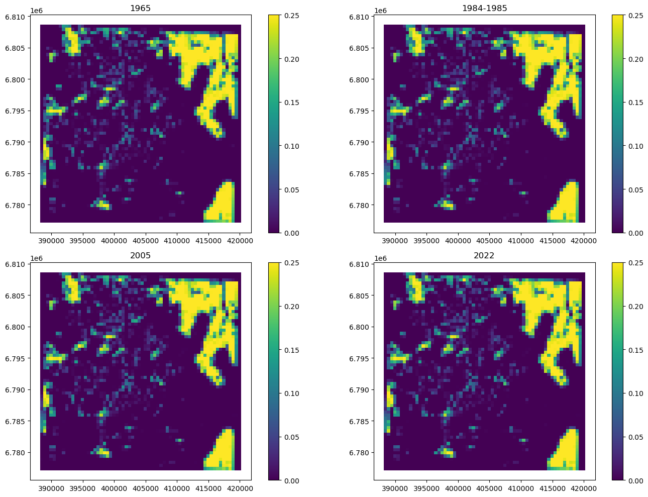
= plt.subplots(2 ,2 , figsize= (14 ,10 ))0 , inplace= True )= 'waterbody_area_65' , ax= axs[0 ,0 ], vmin= 0 , vmax= .500 ** 2 , legend= True ).set_title('1965' )= 'waterbody_area_85' , ax= axs[0 ,1 ], vmin= 0 , vmax= .500 ** 2 , legend= True ).set_title('1984-1985' )= 'waterbody_area_05' , ax= axs[1 ,0 ], vmin= 0 , vmax= .500 ** 2 , legend= True ).set_title('2005' )= 'waterbody_area_22' , ax= axs[1 ,1 ], vmin= 0 , vmax= .500 ** 2 , legend= True ).set_title('2022' )
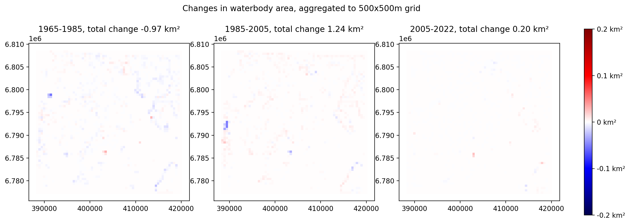
Quantify the change. Negative change means decreased waterbody area.
Code
'waterbody_change_6585' ] = (grid.waterbody_area_85 - grid.waterbody_area_65)'waterbody_change_8505' ] = (grid.waterbody_area_05 - grid.waterbody_area_85)'waterbody_change_0522' ] = (grid.waterbody_area_22 - grid.waterbody_area_05)
Change stats for 1965-1985:
Code
print (f'Gain: { grid[grid.waterbody_change_6585 > 0 ]. waterbody_change_6585. sum ():.2f} km²' )print (f'Loss: { - grid[grid.waterbody_change_6585 < 0 ]. waterbody_change_6585. sum ():.2f} km²' )print (f'Change: { grid. waterbody_change_6585. sum ():.2f} km²' )
Gain: 0.97 km²
Loss: 1.93 km²
Change: -0.97 km²
Change stats for 1985-2005
Code
print (f'Gain: { grid[grid.waterbody_change_8505 > 0 ]. waterbody_change_8505. sum ():.2f} km²' )print (f'Loss: { - grid[grid.waterbody_change_8505 < 0 ]. waterbody_change_8505. sum ():.2f} km²' )print (f'Change: { grid. waterbody_change_8505. sum ():.2f} km²' )
Gain: 2.01 km²
Loss: 0.77 km²
Change: 1.24 km²
Change stats for 2005-2022
Code
print (f'Gain: { grid[grid.waterbody_change_0522 > 0 ]. waterbody_change_0522. sum ():.2f} km²' )print (f'Loss: { - grid[grid.waterbody_change_0522 < 0 ]. waterbody_change_0522. sum ():.2f} km²' )print (f'Change: { grid. waterbody_change_0522. sum ():.2f} km²' )
Gain: 0.38 km²
Loss: 0.18 km²
Change: 0.20 km²
Code
= plt.subplots(1 ,4 , figsize= (15 ,5 ), dpi= 200 , gridspec_kw= {'width_ratios' : [1 ,1 ,1 ,0.05 ]})= 'waterbody_change_6585' , cmap= 'seismic' , vmin=- .20 , vmax= .20 , ax= axs[0 ])= 'waterbody_change_8505' , cmap= 'seismic' , vmin=- .20 , vmax= .20 , ax= axs[1 ])= 'waterbody_change_0522' , cmap= 'seismic' , vmin=- .20 , vmax= .20 , ax= axs[2 ])0 ].set_title(f'1965-1985, total change { grid. waterbody_change_6585. sum ():.2f} km²' )1 ].set_title(f'1985-2005, total change { grid. waterbody_change_8505. sum ():.2f} km²' )2 ].set_title(f'2005-2022, total change { grid. waterbody_change_0522. sum ():.2f} km²' )= colors.Normalize(vmin=- .2 ,vmax= .2 )= plt.cm.ScalarMappable(cmap= 'seismic' , norm= norm)= [- .2 ,- .1 ,0 ,.1 ,.2 ]= plt.colorbar(sm, cax= axs[3 ], ticks= ticks)f' { t} km²' for t in ticks])'Changes in waterbody area, aggregated to 500x500m grid' )
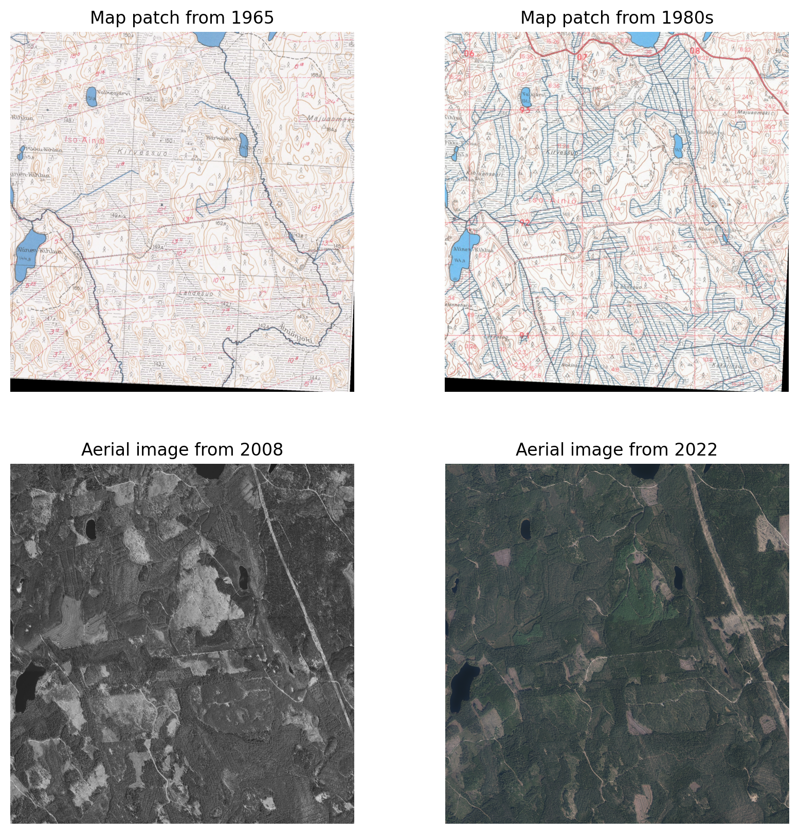
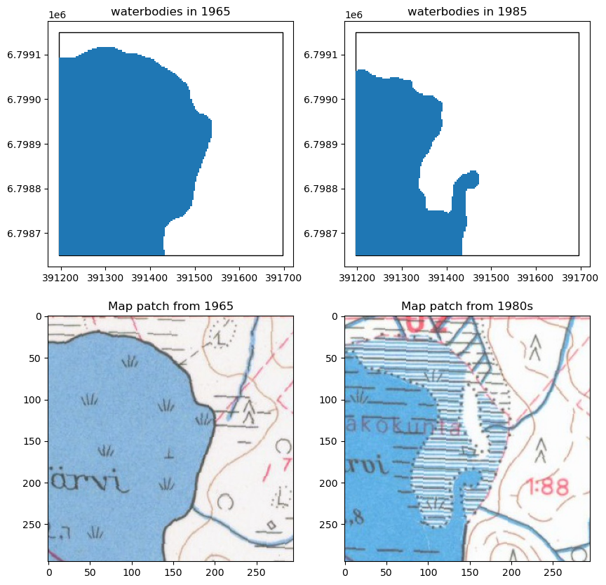
Visualize the location where the waterbody area has decreased the most between 1965 and 1985. For 1965 and 1980s show the corresponding map patch along with the data.
For 2005 and 2022, show the closest aerial image to that year. Unfortunately the closest historical images available are from 1949 and 1979, so we can’t really use them for visualizations.
Code
= grid[grid.waterbody_change_6585 == grid.waterbody_change_6585.min ()].cellid.iloc[0 ]= plt.subplots(2 ,2 , figsize= (10 ,10 ))== waterbodyloss_6585_cellid].plot(ax= axs[0 ,0 ], facecolor= 'none' )== waterbodyloss_6585_cellid].geometry).plot(ax= axs[0 ,0 ], color= 'tab:blue' ).set_title('waterbodies in 1965' )== waterbodyloss_6585_cellid].plot(ax= axs[0 ,1 ], facecolor= 'none' )== waterbodyloss_6585_cellid].geometry).plot(ax= axs[0 ,1 ], color= 'tab:blue' ).set_title('waterbodies in 1985' )= get_map_patch(grid[grid.cellid == waterbodyloss_6585_cellid].geometry.iloc[0 ], 1965 , map_path)1 ,0 ].imshow(img, cmap= 'gray' )1 ,0 ].set_title(f'Map patch from 1965' )= get_map_patch(grid[grid.cellid == waterbodyloss_6585_cellid].geometry.iloc[0 ], 1985 , map_path)1 ,1 ].imshow(img, cmap= 'gray' )1 ,1 ].set_title(f'Map patch from 1980s' )
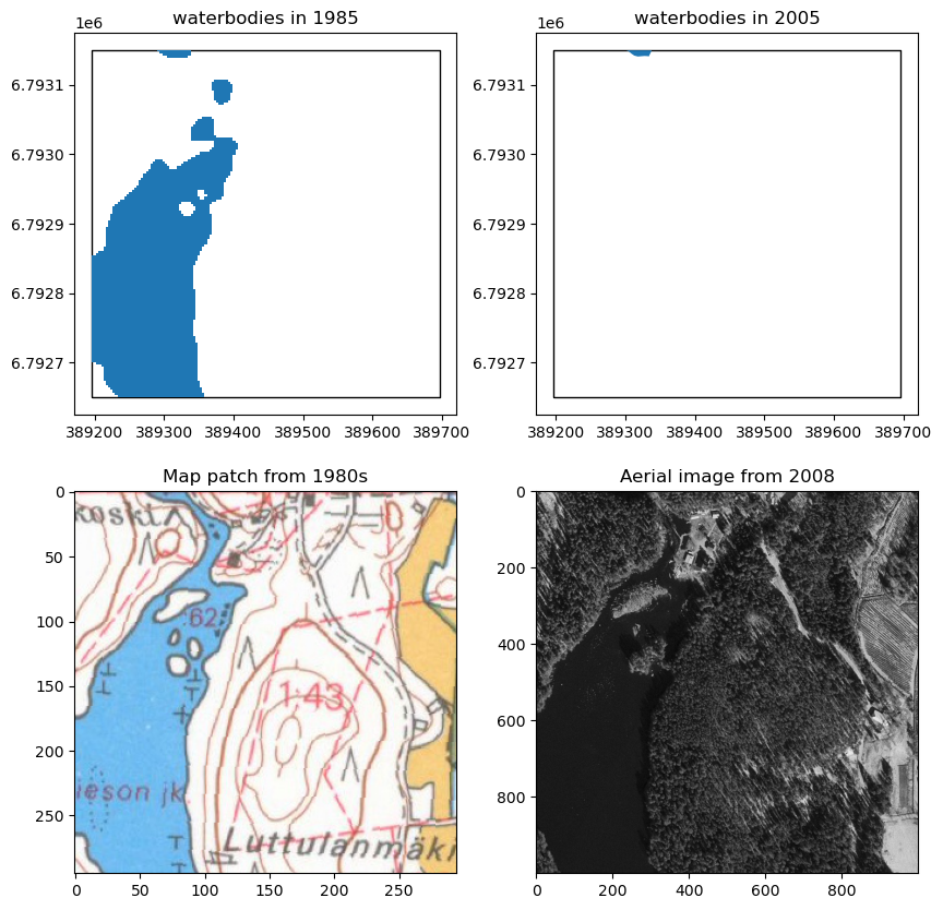
Same for 1985 and 2005
Code
= grid[grid.waterbody_change_8505 == grid.waterbody_change_8505.min ()].cellid.iloc[0 ]= plt.subplots(2 ,2 , figsize= (10 ,10 ))== waterbodyloss_8505_cellid].plot(ax= axs[0 ,0 ], facecolor= 'none' )== waterbodyloss_8505_cellid].geometry).plot(ax= axs[0 ,0 ], color= 'tab:blue' ).set_title('waterbodies in 1985' )== waterbodyloss_8505_cellid].plot(ax= axs[0 ,1 ], facecolor= 'none' )== waterbodyloss_8505_cellid].geometry).plot(ax= axs[0 ,1 ], color= 'tab:blue' ).set_title('waterbodies in 2005' )= get_map_patch(grid[grid.cellid == waterbodyloss_8505_cellid].geometry.iloc[0 ], 1985 , map_path)1 ,0 ].imshow(img, cmap= 'gray' )1 ,0 ].set_title(f'Map patch from 1980s' )= get_wcs_img(grid[grid.cellid == waterbodyloss_8505_cellid].total_bounds, 2005 )1 ,1 ].imshow(img, cmap= 'gray' )1 ,1 ].set_title(f'Aerial image from { year} ' )
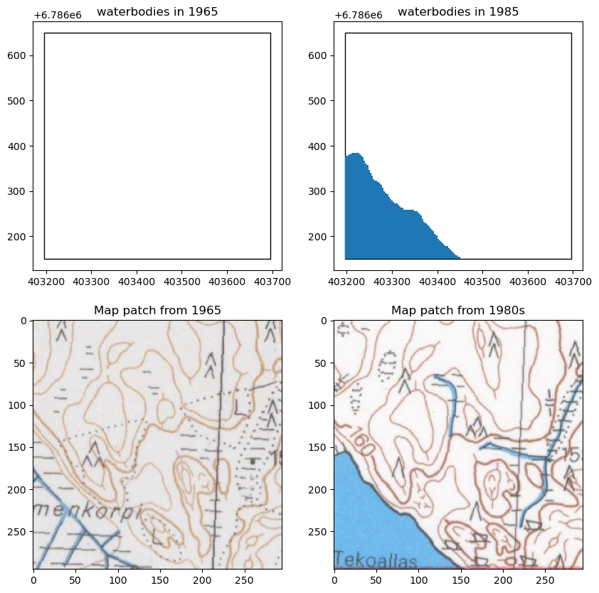
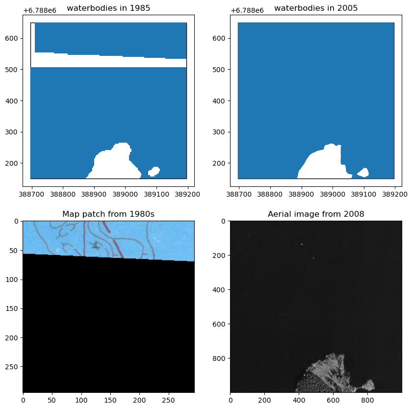
And then same visualizations for waterbody area increase.
Code
= grid[grid.waterbody_change_6585 == grid.waterbody_change_6585.max ()].cellid.iloc[0 ]= plt.subplots(2 ,2 , figsize= (10 ,10 ))== waterbodygain_6585_cellid].plot(ax= axs[0 ,0 ], facecolor= 'none' )== waterbodygain_6585_cellid].geometry).plot(ax= axs[0 ,0 ], color= 'tab:blue' ).set_title('waterbodies in 1965' )== waterbodygain_6585_cellid].plot(ax= axs[0 ,1 ], facecolor= 'none' )== waterbodygain_6585_cellid].geometry).plot(ax= axs[0 ,1 ], color= 'tab:blue' ).set_title('waterbodies in 1985' )= get_map_patch(grid[grid.cellid == waterbodygain_6585_cellid].geometry.iloc[0 ], 1965 , map_path)1 ,0 ].imshow(img, cmap= 'gray' )1 ,0 ].set_title(f'Map patch from 1965' )= get_map_patch(grid[grid.cellid == waterbodygain_6585_cellid].geometry.iloc[0 ], 1985 , map_path)1 ,1 ].imshow(img, cmap= 'gray' )1 ,1 ].set_title(f'Map patch from 1980s' )
Code
= grid[grid.waterbody_change_8505 == grid.waterbody_change_8505.max ()].cellid.iloc[0 ]= plt.subplots(2 ,2 , figsize= (10 ,10 ))== waterbodygain_8505_cellid].plot(ax= axs[0 ,0 ], facecolor= 'none' )== waterbodygain_8505_cellid].geometry).plot(ax= axs[0 ,0 ], color= 'tab:blue' ).set_title('waterbodies in 1985' )== waterbodygain_8505_cellid].plot(ax= axs[0 ,1 ], facecolor= 'none' )== waterbodygain_8505_cellid].geometry).plot(ax= axs[0 ,1 ], color= 'tab:blue' ).set_title('waterbodies in 2005' )= get_map_patch(grid[grid.cellid == waterbodygain_8505_cellid].geometry.iloc[0 ], 1985 , map_path)1 ,0 ].imshow(img, cmap= 'gray' )1 ,0 ].set_title(f'Map patch from 1980s' )= get_wcs_img(grid[grid.cellid == waterbodygain_8505_cellid].total_bounds, 2005 )1 ,1 ].imshow(img, cmap= 'gray' )1 ,1 ].set_title(f'Aerial image from { year} ' )