Extracting colors with simple thresholding

Author

Janne Mäyrä

Published

February 27, 2023

The simplest approach for extracting information is a simple color extraction which can be used to detect land cover classes distinguished by color such as fields and waters. However, textural areas such as marshes can not be detected this way.

All these extractions are done with white-balance corrected images.

Code

import cv2
import numpy as np
import os
from pathlib import Path
import matplotlib.pyplot as plt

Code

datapath = Path('../data/maps/aligned_maps/')
files = sorted(os.listdir(datapath))
ex_file = cv2.imread(str(datapath/files[3]))
plt.imshow(cv2.cvtColor(ex_file, cv2.COLOR_BGR2RGB))
plt.title(files[3])

Text(0.5, 1.0, '213406_1984.tif')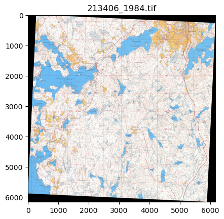

For easier color filtering, images are transformed into HSV colorspace

Code

hsv_ex = cv2.cvtColor(ex_file, cv2.COLOR_BGR2HSV)
plt.imshow(hsv_ex)
plt.title(files[4])

Text(0.5, 1.0, '213408_1965.tif')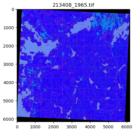

1 Fields

HSV-range for fields is between [10, 100, 100] and [25, 255, 255]

Code

hsv_field_bot = np.array([10,100,100])
hsv_field_top = np.array([25,255,255])
field_mask = cv2.inRange(hsv_ex, hsv_field_bot, hsv_field_top)
field_mask = field_mask.astype(np.int16)
fig, axs = plt.subplots(1,2, figsize=(10,6), dpi=150)
field_mask[field_mask<128] = 0
field_mask[field_mask>128] = 1
axs[0].imshow(field_mask, interpolation='none')
temp = ex_file.copy()
temp[field_mask == 0] = 255
axs[1].imshow(cv2.cvtColor(temp, cv2.COLOR_BGR2RGB))
plt.show()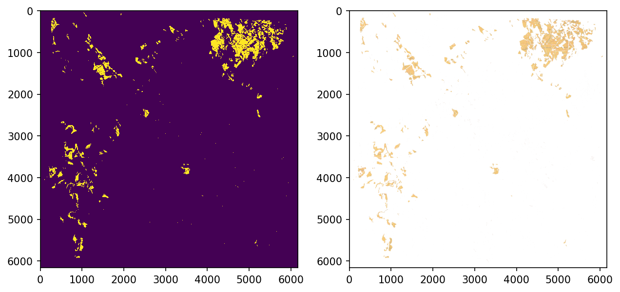

Code

fig, axs = plt.subplots(1, 2, figsize=(10,6), dpi=150)
axs[0].imshow(cv2.cvtColor(ex_file[500:1000, 4000:4500], cv2.COLOR_BGR2RGB))
axs[1].imshow(cv2.cvtColor(temp[500:1000, 4000:4500], cv2.COLOR_BGR2RGB))

<matplotlib.image.AxesImage>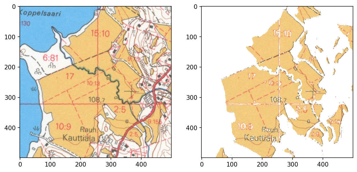

2 Waters

Water range is between [60,10,10] aand [130,255,255].

Code

hsv_water_bot = np.array([60,10,10])
hsv_water_top = np.array([130,255,255])
water_mask = cv2.inRange(hsv_ex, hsv_water_bot, hsv_water_top)
water_mask = water_mask.astype(np.uint8)
water_mask = water_mask
fig, axs = plt.subplots(1,2, figsize=(10,6), dpi=200)
water_mask[water_mask<128] = 0
water_mask[water_mask>128] = 1
axs[0].imshow(water_mask, interpolation='none')
temp = ex_file.copy()
temp[water_mask == 0] = 255
axs[1].imshow(cv2.cvtColor(temp, cv2.COLOR_BGR2RGB), interpolation='none')
plt.show()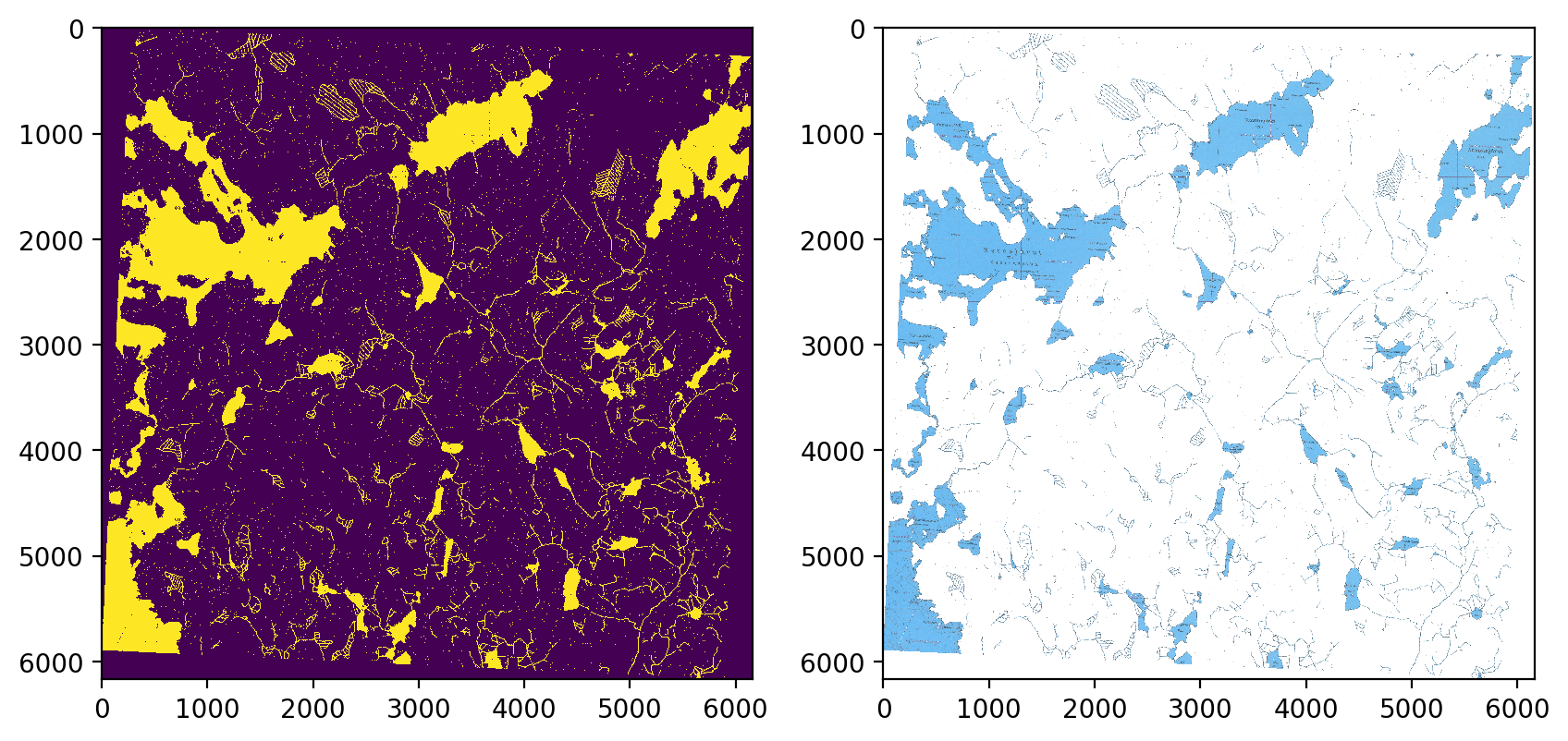

This approach, however, has some difficulties with ditches running through fields as their color is greenish rather than blue.

Code

fig, axs = plt.subplots(1, 2, figsize=(10,6), dpi=150)
axs[0].imshow(cv2.cvtColor(ex_file[500:1000, 4000:4500], cv2.COLOR_BGR2RGB))
axs[1].imshow(cv2.cvtColor(temp[500:1000, 4000:4500], cv2.COLOR_BGR2RGB))

<matplotlib.image.AxesImage>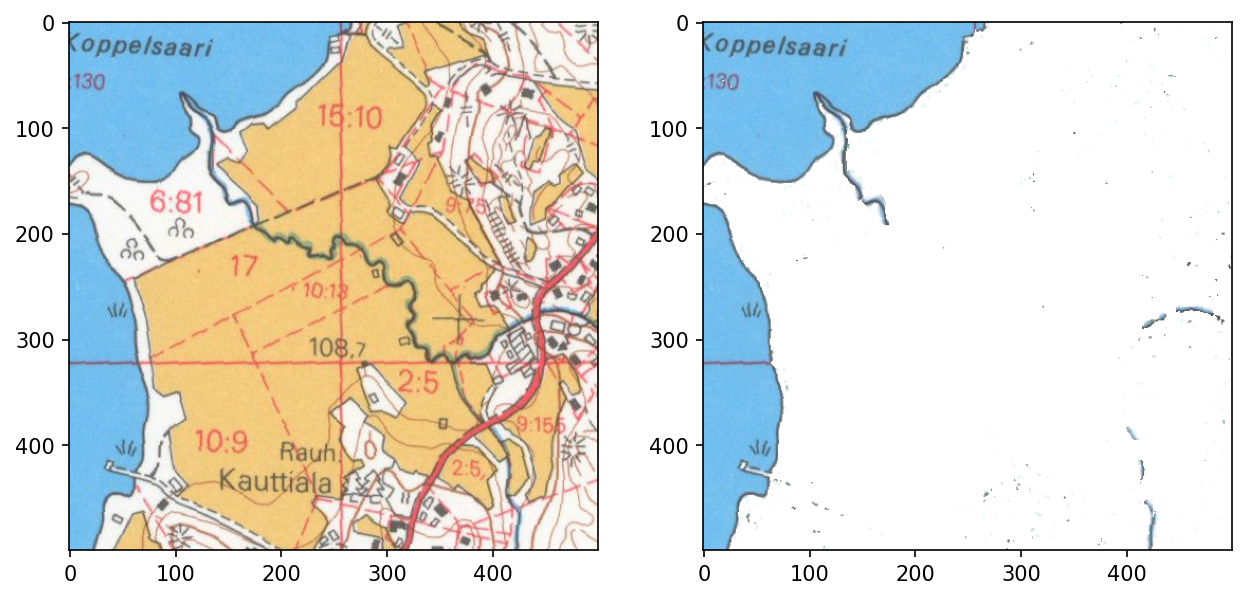

Also, overlapping colors are fairly difficult situations.

Code

fig, axs = plt.subplots(1, 2, figsize=(10,6), dpi=150)
axs[0].imshow(cv2.cvtColor(ex_file[500:1500, 2000:3000], cv2.COLOR_BGR2RGB))
axs[1].imshow(cv2.cvtColor(temp[500:1500, 2000:3000], cv2.COLOR_BGR2RGB))

<matplotlib.image.AxesImage>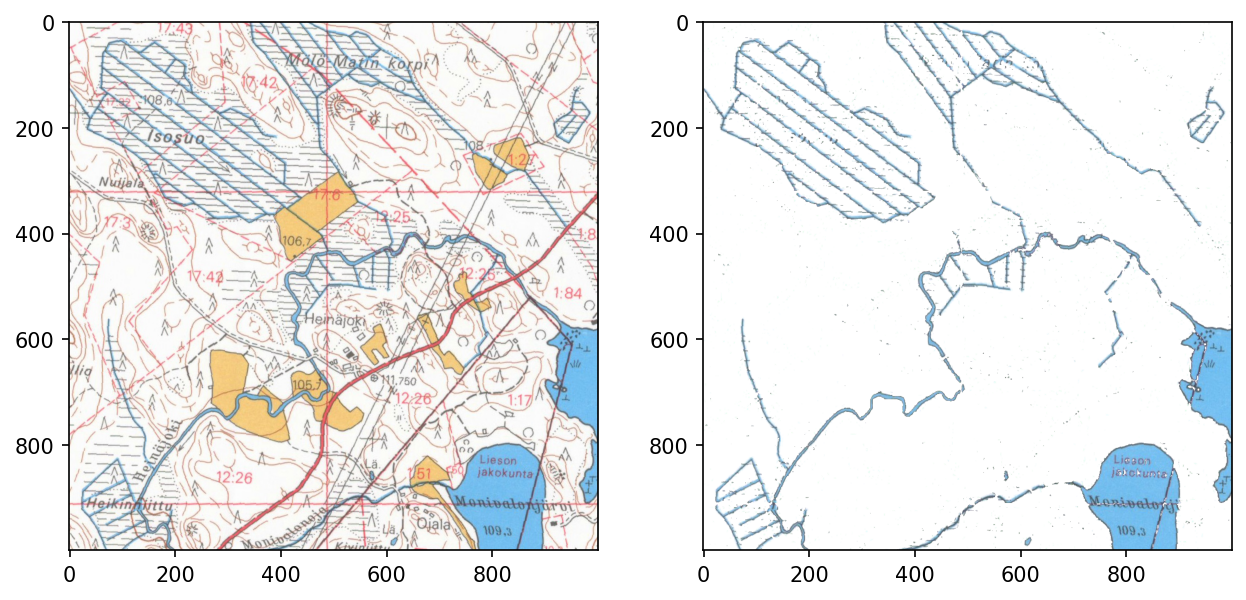

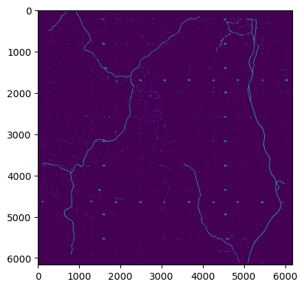
Distinguishing between water bodies and waterways can be done fairly easily with MORPH_OPEN.

Code

water_mask_open = cv2.morphologyEx(water_mask, cv2.MORPH_OPEN, cv2.getStructuringElement(cv2.MORPH_RECT, (15,15)))
fig, axs = plt.subplots(1, 3, dpi=200, figsize=(10,6))
axs[0].imshow(water_mask[500:1500, 2000:3000])
axs[0].set_title('Blue mask')
axs[1].imshow(water_mask_open[500:1500, 2000:3000])
axs[1].set_title('Water bodies')
axs[2].imshow((water_mask - water_mask_open)[500:1500, 2000:3000])
axs[2].set_title('Waterways')

Text(0.5, 1.0, 'Waterways')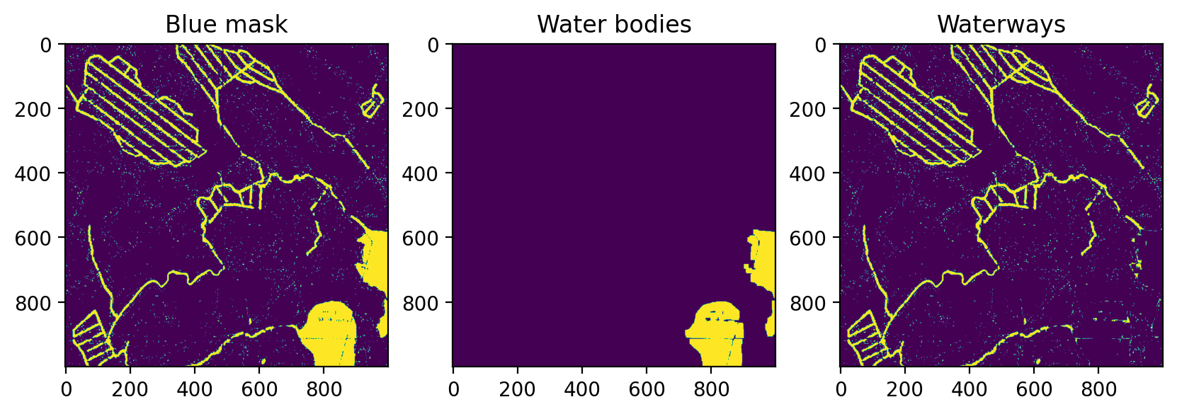

After some post-processing the waterway-layer looks fairly good.

Code

from skimage.morphology import skeletonize

fig, axs = plt.subplots(1,3, dpi=200, figsize=(10,4))
for a in axs:
    a.set_xticks([])
    a.set_yticks([])

waterways = (water_mask - water_mask_open)[500:1500, 2000:3000]
axs[0].imshow(waterways)
axs[0].set_title('Waterways')
opened = cv2.morphologyEx(waterways, cv2.MORPH_OPEN, cv2.getStructuringElement(cv2.MORPH_CROSS, (5,5)))
axs[1].imshow(opened)
axs[1].set_title('Opening with 5x5 kernel')
axs[2].imshow(skeletonize(opened))
axs[2].set_title('Skeletonized waterways')

Text(0.5, 1.0, 'Skeletonized waterways')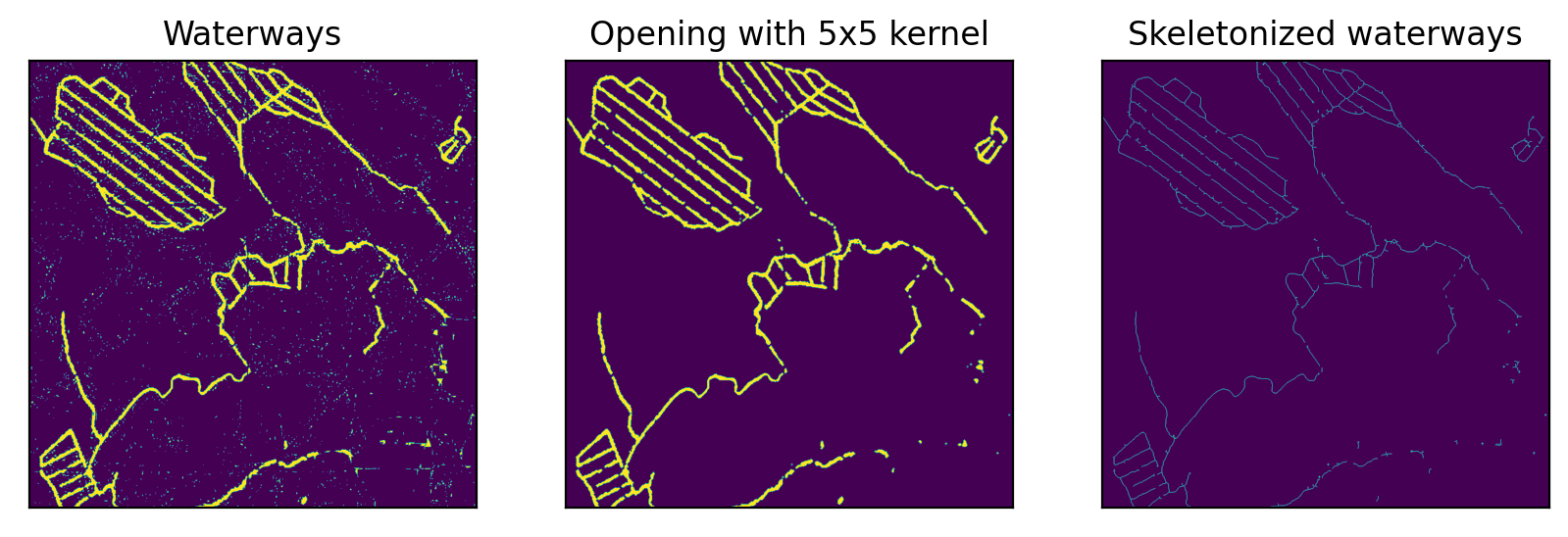

3 Roads

As red wraps around 180 in HSV-colorspace, two ranges are required for it.

Code

hsv_red_bot1 = np.array([0,10,10])
hsv_red_top1 = np.array([5,255,255])
hsv_red_bot2 = np.array([175,10,10])
hsv_red_top2 = np.array([180,255,255])
red_mask1 = cv2.inRange(hsv_ex, hsv_red_bot1, hsv_red_top1)
red_mask1 = red_mask1.astype(np.int16)
red_mask2 = cv2.inRange(hsv_ex, hsv_red_bot2, hsv_red_top2)
red_mask2 = red_mask2.astype(np.int16)
fig, axs = plt.subplots(1,2, figsize=(10,6), dpi=150)
red_mask = red_mask1 | red_mask2
red_mask[red_mask<128] = 0
red_mask[red_mask>128] = 1
axs[0].imshow(red_mask, interpolation='none')
temp = ex_file.copy()
temp[red_mask == 0] = 255
axs[1].imshow(cv2.cvtColor(temp, cv2.COLOR_BGR2RGB))
plt.show()

Another approach is to invert the RGB-image, convert it to HSV and look for cyan.

Code

plt.imshow(cv2.cvtColor(~ex_file, cv2.COLOR_BGR2RGB))

<matplotlib.image.AxesImage>

Code

inv_hsv = cv2.cvtColor(~ex_file, cv2.COLOR_BGR2HSV)
hsv_cyan_bot = np.array([85,70,50])
hsv_cyan_top = np.array([95,255,255])
cyan_mask = cv2.inRange(inv_hsv, hsv_cyan_bot, hsv_cyan_top)
cyan_mask = cyan_mask.astype(np.uint8)
fig, axs = plt.subplots(1,2, figsize=(10,6), dpi=150)
cyan_mask[cyan_mask<128] = 0
cyan_mask[cyan_mask>128] = 1
axs[0].imshow(cyan_mask, interpolation='none')
temp = ex_file.copy()
temp[cyan_mask == 0] = 255
axs[1].imshow(cv2.cvtColor(temp, cv2.COLOR_BGR2RGB))
plt.show()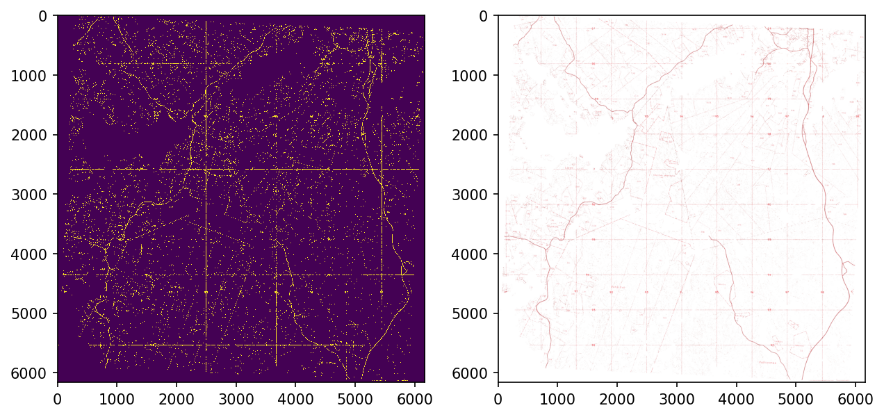

Unfortunately, there are lots of other things than roads that are red in the images. We can get rid of some of them with simple morphological opening but not nearly all of them.

Code

kernel = cv2.getStructuringElement(cv2.MORPH_RECT, (5,5))
opened = cv2.morphologyEx(cyan_mask, cv2.MORPH_OPEN, kernel)
plt.imshow(opened)

<matplotlib.image.AxesImage>