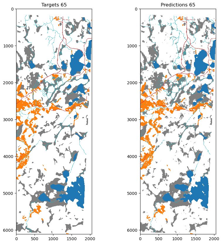
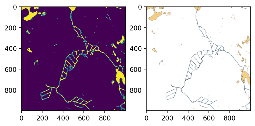
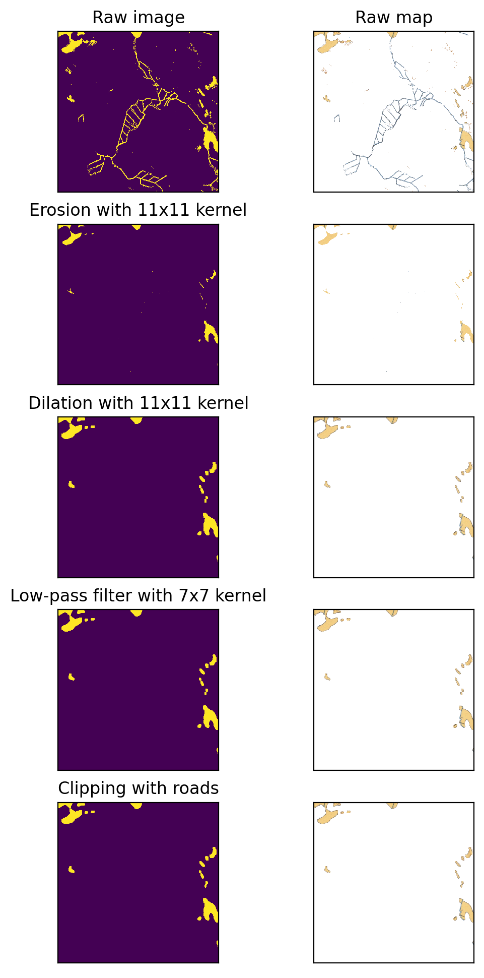
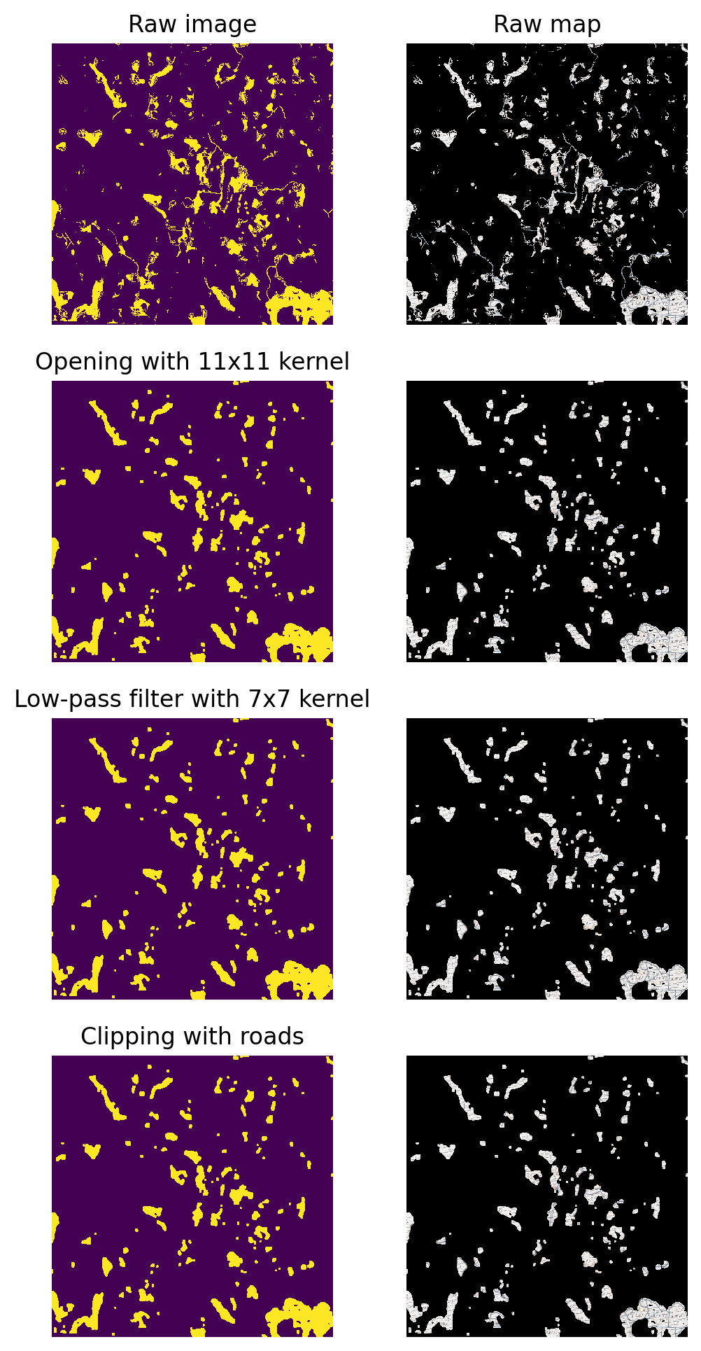
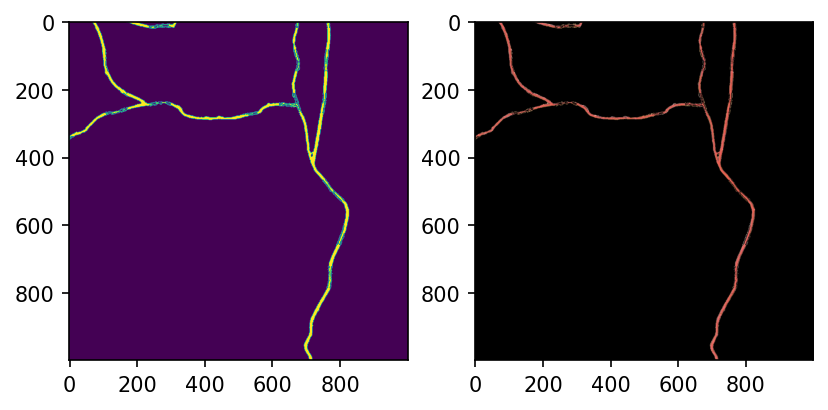
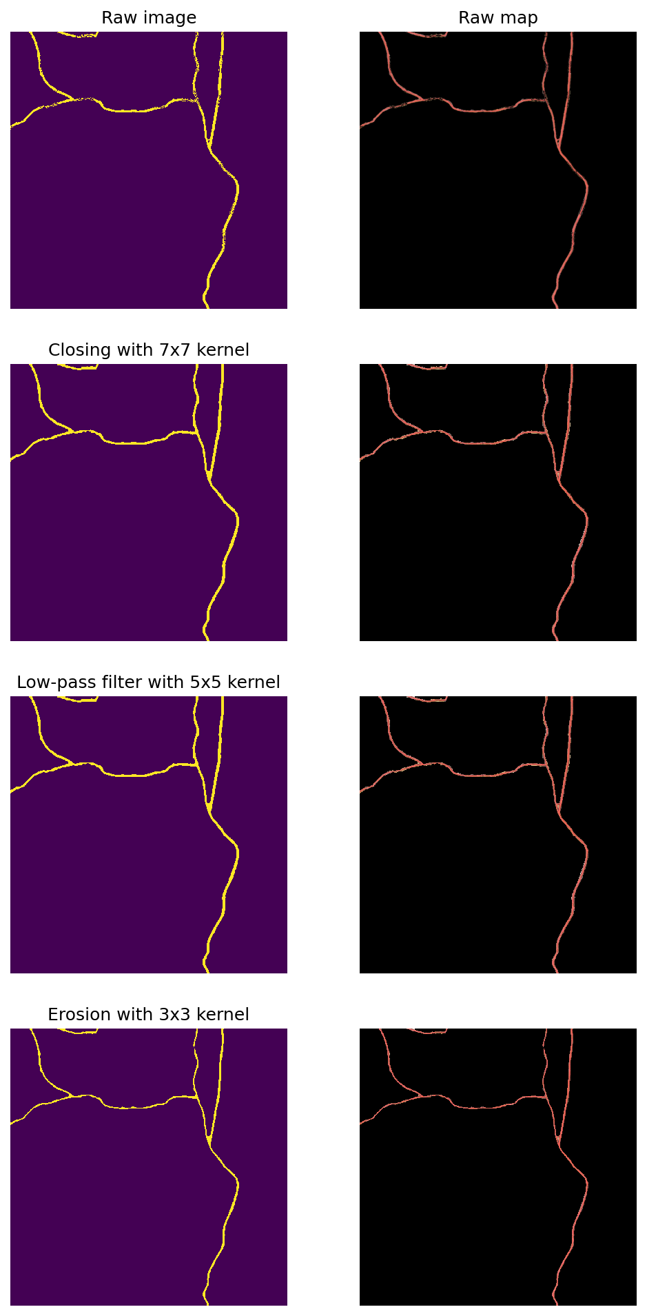
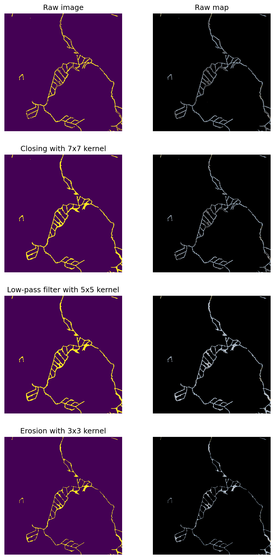
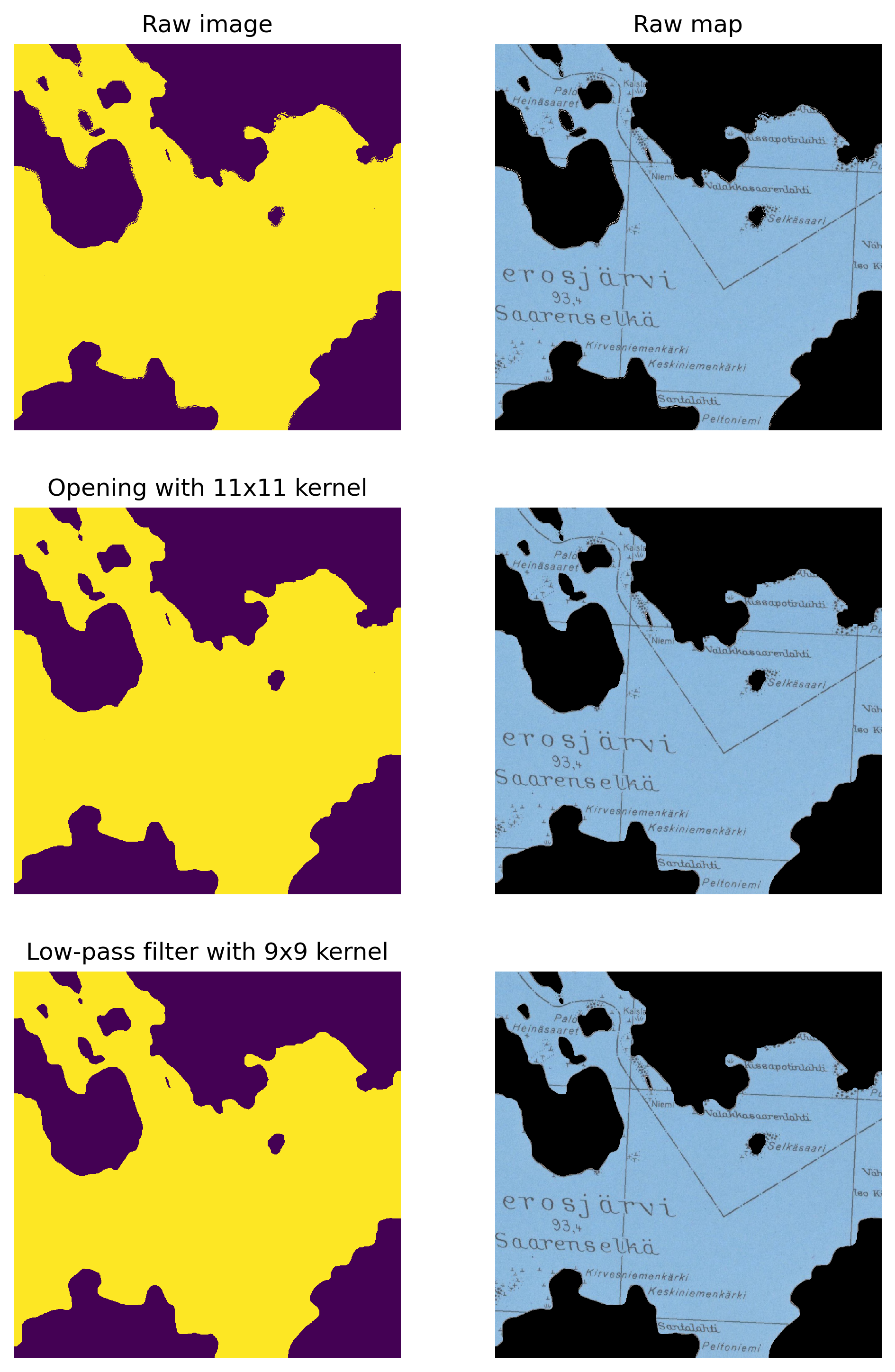
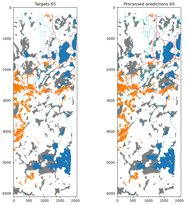
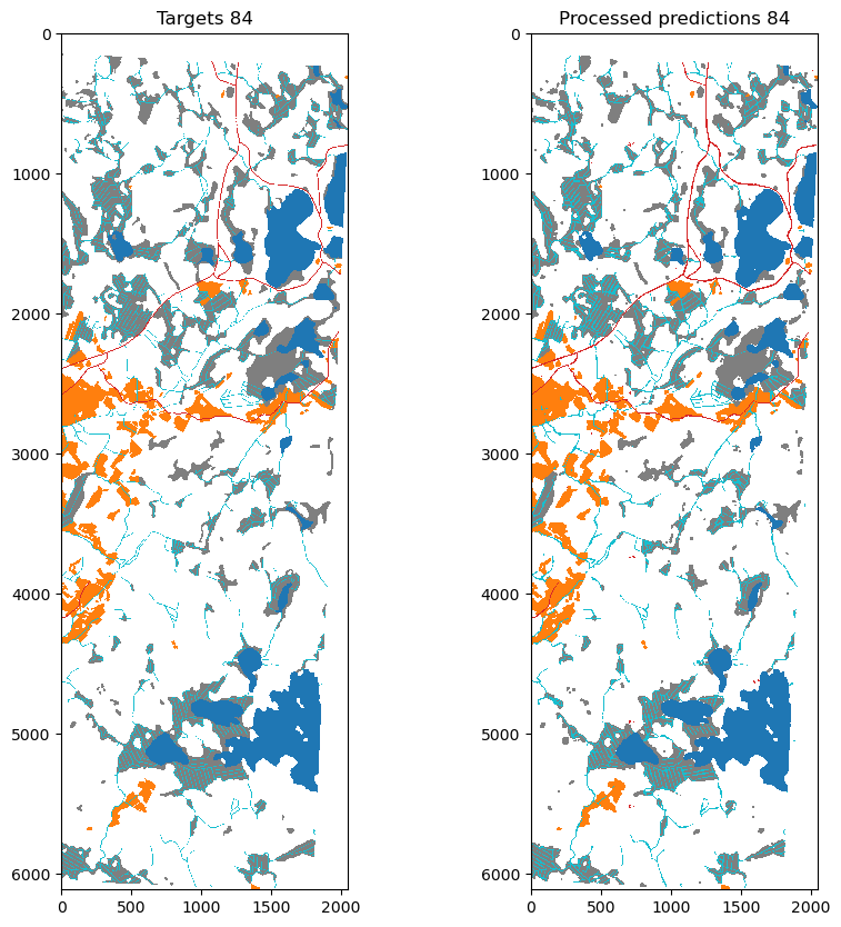
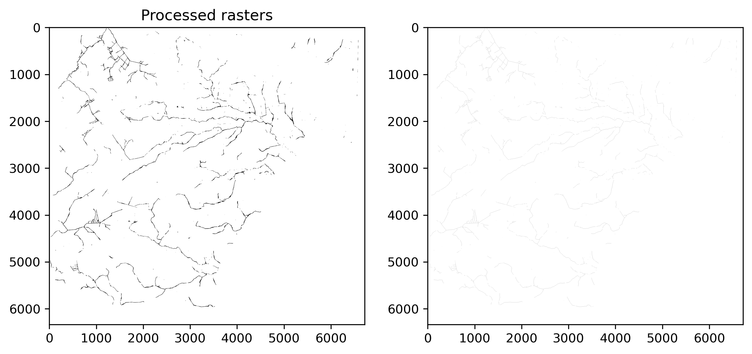
We then used the model trained previously to classify all historical maps from our study area. In order to reduce noise and make predictions smoother, some post-processing steps are required. For this, we used morphological operations such as closing, and erosion, as well as low-pass filtering with suitable kernel sizes.
Code
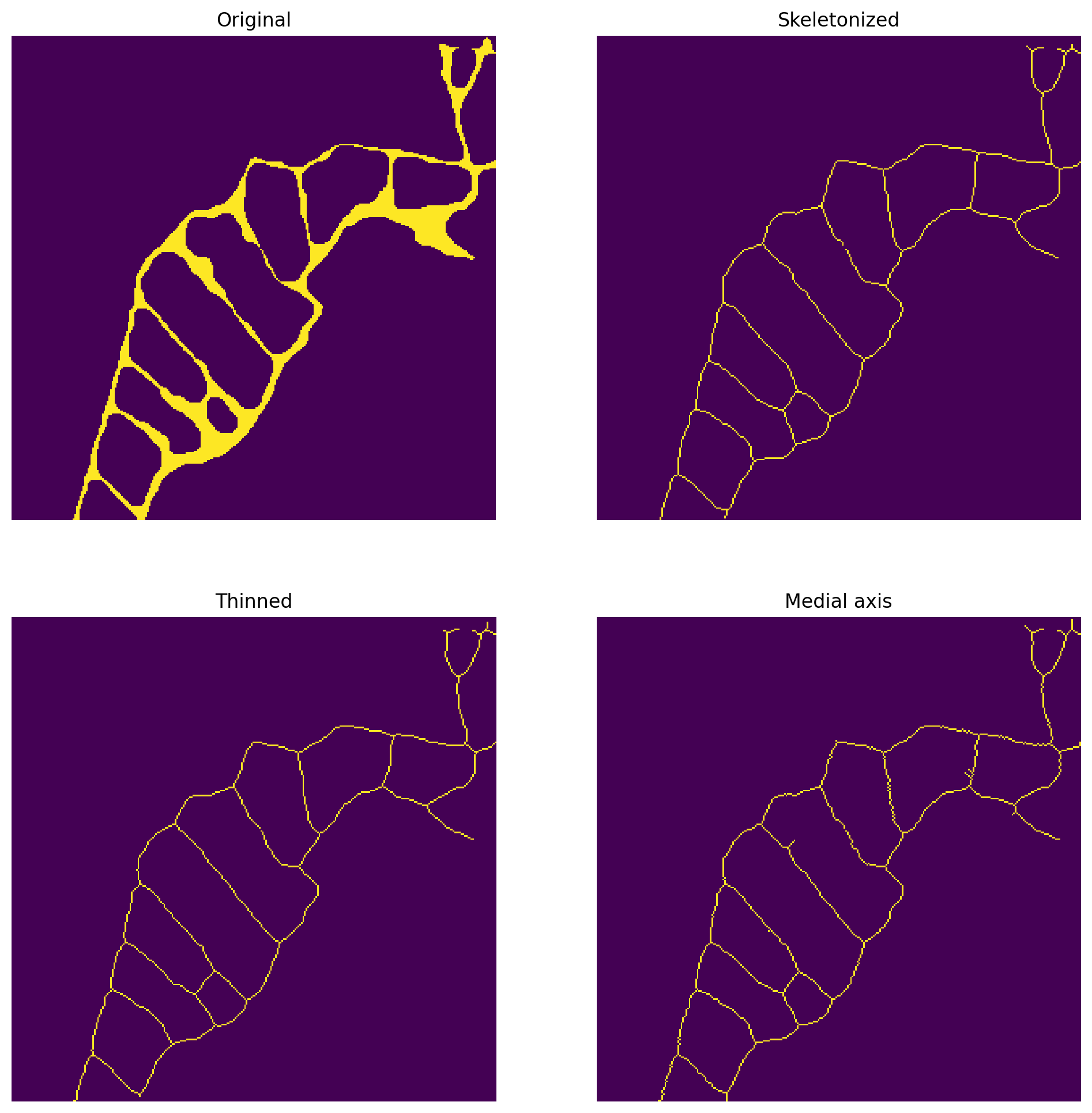
import cv2import numpy as npimport rasterio as rioimport matplotlib.pyplot as pltimport numpy as npimport geopandas as gpdimport rasterio.mask as rio_maskfrom shapely.geometry import boxfrom pathlib import Pathimport osfrom tqdm import tqdmimport fionafrom rasterio import featuresfrom rasterio.enums import Resamplingfrom itertools import productfrom shapely.geometry import Polygonfrom skimage.morphology import skeletonize, medial_axis, thin
Code
def polygonize(fn, outpath, target_class, scale_factor=1):with rio.open(fn) as src: im = src.read(out_shape=(src.count, int(src.height*scale_factor),int(src.width*scale_factor)), resampling=Resampling.mode)[target_class -1] im[im !=0] =1 mask = im ==1 tfm = src.transform * src.transform.scale((src.width/im.shape[-1]), (src.height/im.shape[-2])) results = ({'properties': {'raster_val': v}, 'geometry': s}for i, (s, v) inenumerate(features.shapes(im, mask==mask, transform=tfm))if v ==1)with fiona.open(outpath, 'w', driver='GeoJSON', crs='EPSG:3067', schema={'properties': [('raster_val', 'int')],'geometry': 'Polygon'}) as dst: dst.writerecords(results)
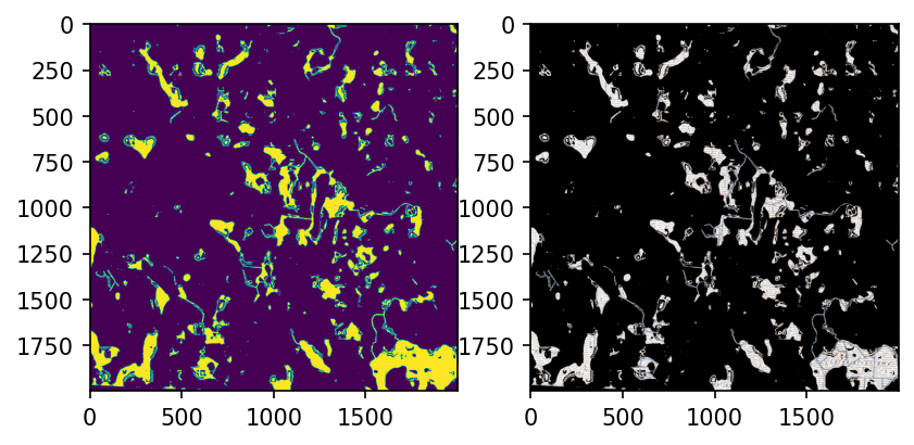
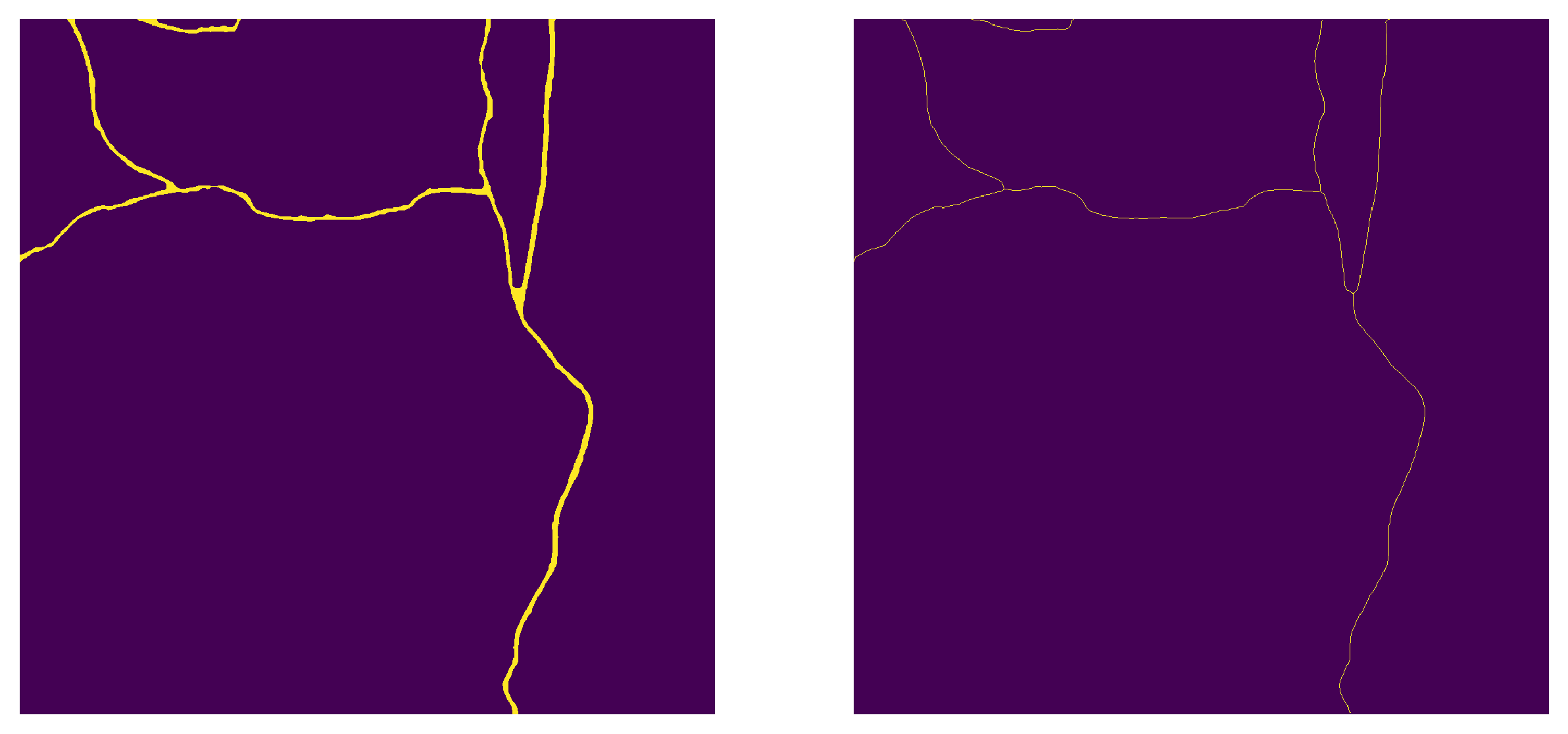
The postprocessing steps depend on the land cover class and how they are layered in the final products. Roads and watercourses are such classes that the final products for these are line geometries, whereas the other classes can be either raster data or polygon data. Most watercourses (e.g. ditches) do not split mires and fields into multiple sections, whereas roads split these classes into multiple different segments.
Code
ex_data ='../results/raw/213406_1965_ei_rajoja.tif'with rio.open(ex_data) as src: data = src.read(1)ex_map ='../data/maps/aligned_maps/213406_1965_ei_rajoja.tif'with rio.open(ex_map) as src: mapdata = np.moveaxis(src.read(), 0, -1)mapdata = mapdata[32:, 32:] data = data[:mapdata.shape[0], :mapdata.shape[1]]
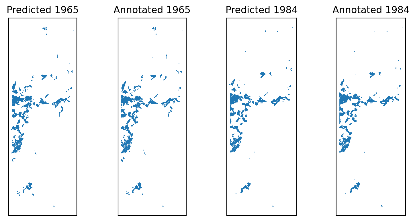
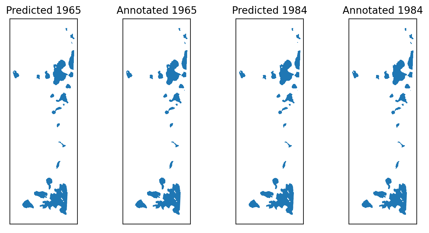
2.1 Fields
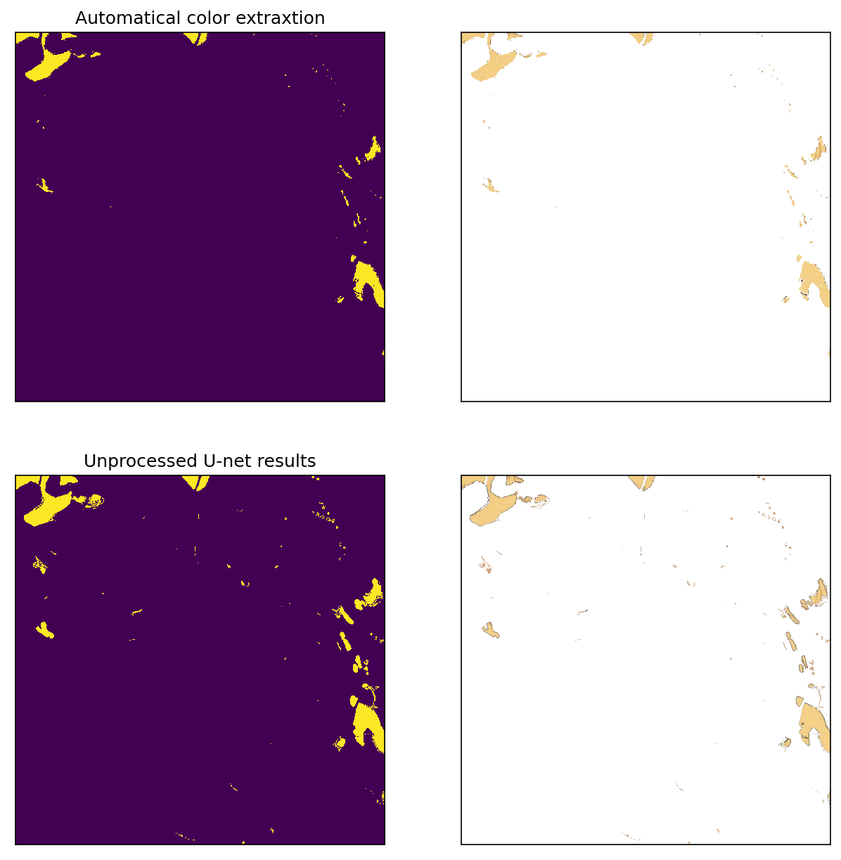
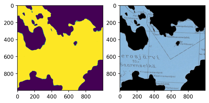
Comparison with automatically extracted orange color.
During postprocessing, include watercourses for these layers. MORPH.OPEN (erosion followed by dilation) with 11x11 kernel is sufficient to remove watercourses from non-field areas.
for r in ['213405_1965.tif', '213405_1984.tif']: polygonize(respath/r, polypath/'fields'/r.replace('tif', 'geojson'), target_class=1, scale_factor=1/2)for r in ['val_mask_1965.tif', 'val_mask_1984.tif']: polygonize(refpath/'postproc'/r, refpath/'polydata/fields'/r.replace('tif', 'geojson'), target_class=1, scale_factor=1/2)
print(f'Total predicted field area in 1965: {pred_fields_65.area.sum()*10**-6:.3f} km²')print(f'Total annotated field area in 1965: {ref_fields_65.area.sum()*10**-6:.3f} km²')print(f'Difference in km²: {(pred_fields_65.area.sum()*10**-6- ref_fields_65.area.sum()*10**-6):.3f} km²')print(f'%-difference: {100*(pred_fields_65.area.sum()*10**-6- ref_fields_65.area.sum()*10**-6)/(ref_fields_65.area.sum()*10**-6):.3f} %')
Total predicted field area in 1965: 2.072 km²
Total annotated field area in 1965: 2.102 km²
Difference in km²: -0.030 km²
%-difference: -1.409 %
Code
print(f'Total predicted field area in 1984: {pred_fields_84.area.sum()*10**-6:.3f} km²')print(f'Total annotated field area in 1984: {ref_fields_84.area.sum()*10**-6:.3f} km²')print(f'Difference in km²: {(pred_fields_84.area.sum()*10**-6- ref_fields_84.area.sum()*10**-6):.3f} km²')print(f'%-difference: {100*(pred_fields_84.area.sum()*10**-6- ref_fields_84.area.sum()*10**-6)/(ref_fields_84.area.sum()*10**-6):.3f} %')
Total predicted field area in 1984: 1.749 km²
Total annotated field area in 1984: 1.769 km²
Difference in km²: -0.020 km²
%-difference: -1.120 %
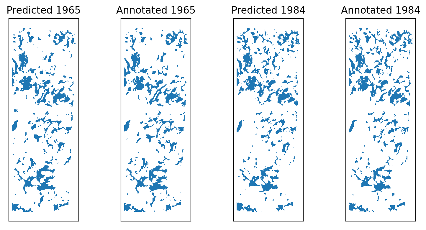
5.2 Mires
Code
for r in ['213405_1965.tif', '213405_1984.tif']: polygonize(respath/r, polypath/'mires'/r.replace('tif', 'geojson'), target_class=2, scale_factor=1/2)for r in ['val_mask_1965.tif', 'val_mask_1984.tif']: polygonize(refpath/'postproc'/r, refpath/'polydata/mires'/r.replace('tif', 'geojson'), target_class=2, scale_factor=1/2)
print(f'Total predicted mire area in 1965: {pred_mires_65.area.sum()*10**-6:.3f} km²')print(f'Total annotated mire area in 1965: {ref_mires_65.area.sum()*10**-6:.3f} km²')print(f'Difference in km²: {(pred_mires_65.area.sum()*10**-6- ref_mires_65.area.sum()*10**-6):.3f} km²')print(f'%-difference: {100*(pred_mires_65.area.sum()*10**-6- ref_mires_65.area.sum()*10**-6)/(ref_mires_65.area.sum()*10**-6):.3f} %')
Total predicted mire area in 1965: 5.789 km²
Total annotated mire area in 1965: 5.919 km²
Difference in km²: -0.129 km²
%-difference: -2.182 %
Code
print(f'Total predicted mire area in 1984: {pred_mires_84.area.sum()*10**-6:.3f} km²')print(f'Total annotated mire area in 1984: {ref_mires_84.area.sum()*10**-6:.3f} km²')print(f'Difference in km²: {(pred_mires_84.area.sum()*10**-6- ref_mires_84.area.sum()*10**-6):.3f} km²')print(f'%-difference: {100*(pred_mires_84.area.sum()*10**-6- ref_mires_84.area.sum()*10**-6)/(ref_mires_84.area.sum()*10**-6):.3f} %')
Total predicted mire area in 1984: 5.804 km²
Total annotated mire area in 1984: 6.001 km²
Difference in km²: -0.196 km²
%-difference: -3.270 %
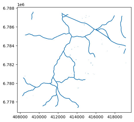
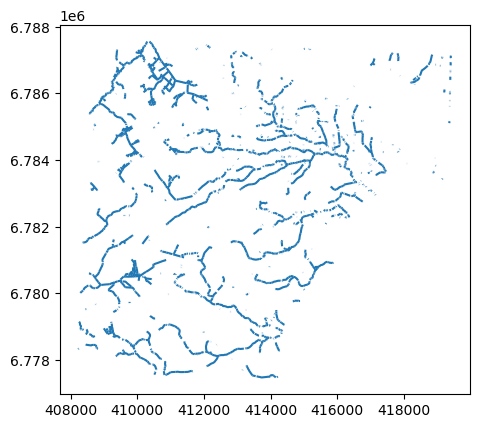
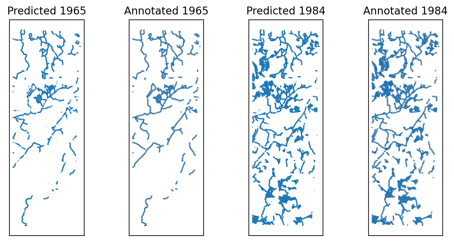
print(f'Total predicted watercourse length in 1965: {pred_watercourses_65.length.sum()*10**-3:.3f} km')print(f'Total annotated watercourse length in 1965: {ref_watercourses_65.length.sum()*10**-3:.3f} km')print(f'Difference in km: {(ref_watercourses_65.length.sum()*10**-3- pred_watercourses_65.length.sum()*10**-3):.3f} km')print(f'%-difference: {100*(ref_watercourses_65.length.sum()*10**-3- pred_watercourses_65.length.sum()*10**-3)/(ref_watercourses_65.length.sum()*10**-3):.3f} %')
Total predicted watercourse length in 1965: 55.786 km
Total annotated watercourse length in 1965: 59.255 km
Difference in km: 3.469 km
%-difference: 5.854 %
Code
print(f'Total predicted watercourse length in 1984: {pred_watercourses_84.length.sum()*10**-3:.3f} km')print(f'Total annotated watercourse length in 1984: {ref_watercourses_84.length.sum()*10**-3:.3f} km')print(f'Difference in km: {(ref_watercourses_84.length.sum()*10**-3- pred_watercourses_84.length.sum()*10**-3):.3f} km')print(f'%-difference: {100*(ref_watercourses_84.length.sum()*10**-3- pred_watercourses_84.length.sum()*10**-3)/(ref_watercourses_84.length.sum()*10**-3):.3f} %')
Total predicted watercourse length in 1984: 160.470 km
Total annotated watercourse length in 1984: 164.801 km
Difference in km: 4.332 km
%-difference: 2.628 %
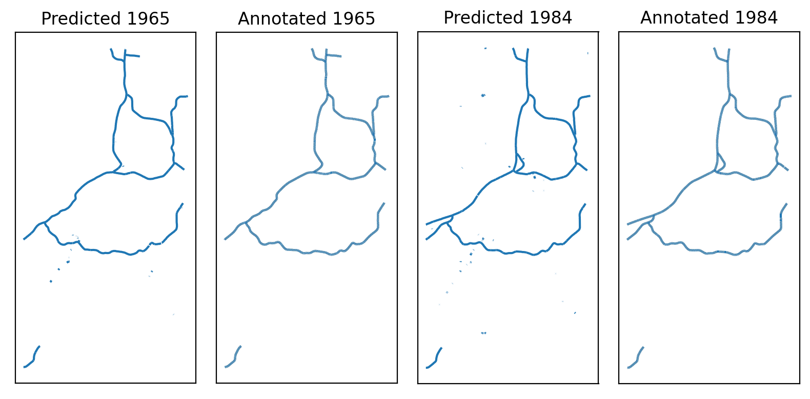
5.5 Water bodies
Code
for r in ['213405_1965.tif', '213405_1984.tif']: polygonize(respath/r, polypath/'water_bodies'/r.replace('tif', 'geojson'), target_class=5, scale_factor=1/2)for r in ['val_mask_1965.tif', 'val_mask_1984.tif']: polygonize(refpath/'postproc'/r, refpath/'polydata/water_bodies'/r.replace('tif', 'geojson'), target_class=5, scale_factor=1/2)
print(f'Total predicted water body area in 1965: {pred_water_bodies_65.area.sum()*10**-6:.3f} km²')print(f'Total annotated water body area in 1965: {ref_water_bodies_65.area.sum()*10**-6:.3f} km²')print(f'Difference in km²: {(ref_water_bodies_65.area.sum()*10**-6- pred_water_bodies_65.area.sum()*10**-6):.3f} km²')print(f'%-difference: {100*(ref_water_bodies_65.area.sum()*10**-6- pred_water_bodies_65.area.sum()*10**-6)/(ref_water_bodies_65.area.sum()*10**-6):.3f} %')
Total predicted water body area in 1965: 2.519 km²
Total annotated water body area in 1965: 2.530 km²
Difference in km²: 0.011 km²
%-difference: 0.449 %
Code
print(f'Total predicted water body area in 1984: {pred_water_bodies_84.area.sum()*10**-6:.3f} km²')print(f'Total annotated water body area in 1984: {ref_water_bodies_84.area.sum()*10**-6:.3f} km²')print(f'Difference in km²: {(ref_water_bodies_84.area.sum()*10**-6- pred_water_bodies_84.area.sum()*10**-6):.3f} km²')print(f'%-difference: {100*(ref_water_bodies_84.area.sum()*10**-6- pred_water_bodies_84.area.sum()*10**-6)/(ref_water_bodies_84.area.sum()*10**-6):.3f} %')
Total predicted water body area in 1984: 2.463 km²
Total annotated water body area in 1984: 2.462 km²
Difference in km²: -0.002 km²
%-difference: -0.069 %