Mask R-CNN model training

Code

import detectron2
from drone_detector.imports import *

from detectron2 import model_zoo
from detectron2.engine import DefaultPredictor
from detectron2.config import get_cfg
from detectron2.utils.visualizer import Visualizer
from detectron2.data import MetadataCatalog, DatasetCatalog, build_detection_test_loader, build_detection_train_loader, DatasetMapper

from detectron2.data import transforms as T
from detectron2.data import detection_utils as utils
import torch

from detectron2.data.datasets import register_coco_instances
from detectron2.engine import DefaultTrainer

from detectron2.evaluation import COCOEvaluator, DatasetEvaluators
import cv2
import matplotlib.pyplot as plt
import wandb

from drone_detector.engines.detectron2.augmentations import *

1 Model training

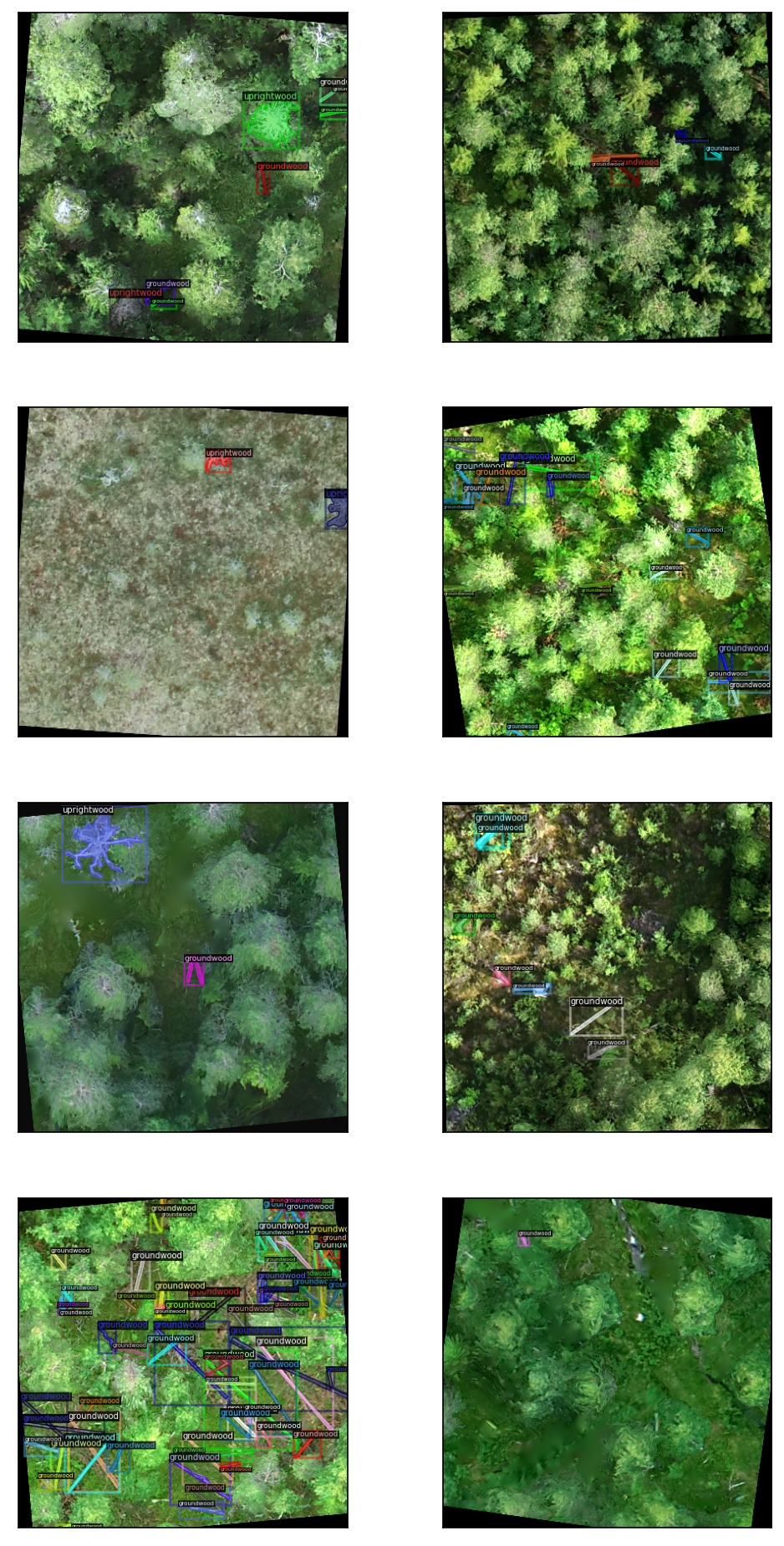
We used Mask R-CNN with a several pretrained backbones as our model, and fine-tuned the model with our remote sensing data. Because the convolutional layers of a CNN model extract interesting, useful features from the images, it is possible and advisable to use pretrained weights as a baseline and fine-tune the model with custom data. All models were trained for 3000 iterations with a batch size of 8, and validation metrics were recorded every 100 iterations. We used a base learning rate of 0.001 and linear warmup with cosine annealing as the learning rate scheduler, using 1000 iterations for the warmup phase.

Code

outpath = Path('../../data/processed/hiidenportti/')
register_coco_instances('hiidenportti_train', {}, outpath/'hiidenportti_train.json', outpath/'train_512')
register_coco_instances('hiidenportti_val', {}, outpath/'hiidenportti_valid.json', outpath/'valid_512')

Code

cfg = get_cfg()
cfg.merge_from_file(model_zoo.get_config_file("COCO-InstanceSegmentation/mask_rcnn_R_50_FPN_3x.yaml"))
cfg.DATASETS.TRAIN = ("hiidenportti_train",)
cfg.DATASETS.TEST = ("hiidenportti_val",)
cfg.DATALOADER.NUM_WORKERS = 4
cfg.MODEL.WEIGHTS = model_zoo.get_checkpoint_url("COCO-InstanceSegmentation/mask_rcnn_R_50_FPN_3x.yaml")  # Let training initialize from model zoo
cfg.SOLVER.IMS_PER_BATCH = 8
cfg.TEST.EVAL_PERIOD = 100
cfg.MODEL.ROI_HEADS.SCORE_THRESH_TEST = 0.5
cfg.OUTPUT_DIR = 'detectron2_models/mask_rcnn_R_50_FPN_3x_256'

cfg.SOLVER.LR_SCHEDULER_NAME = "WarmupCosineLR"
cfg.SOLVER.BASE_LR = 0.001  # pick a good LR
cfg.SOLVER.WARMUP_ITERS = 1000
cfg.SOLVER.MAX_ITER = 3000 
cfg.MODEL.ROI_HEADS.BATCH_SIZE_PER_IMAGE = 512   # (default: 512)
cfg.MODEL.ROI_HEADS.NUM_CLASSES = 2

os.makedirs(cfg.OUTPUT_DIR, exist_ok=True)

Code

class Trainer(DefaultTrainer):
    """
    Trainer class for training detectron2 models
    """
    
    def __init__(self, cfg):
        super().__init__(cfg)
    
    @classmethod
    def build_evaluator(cls, cfg, dataset_name, output_folder=None):
        return DatasetEvaluators([COCOEvaluator(dataset_name, output_dir=output_folder)])
    
    @classmethod
    def build_train_loader(cls, cfg):
        augs = build_aug_transforms(cfg,
                                    flip_horiz=True,
                                    flip_vert=True,
                                    max_rotate=10,
                                    brightness_limits=(.8,1.4),
                                    contrast_limits=(.8,1.4),
                                    saturation_limits=(.8,1.4),
                                    p_lighting=0.75)
        return build_detection_train_loader(cfg, mapper=DatasetMapper(cfg, is_train=True, augmentations=augs))

In order to effectively increase the amount of our training data, we applied a set of augmentations to our image patches and masks. First, each image was randomly flipped and randomly rotated up to 90 degrees. These geometric transformations were applied to both masks and image patches. In addition, brightness and contrast of the image were randomly adjusted and images had a chance to be slightly blurred. Each of these individual augmentations had a probability of 0.5 to be applied.

Code

fig, axs = plt.subplots(4,2, figsize=(8,16), dpi=150)
metadata = MetadataCatalog.get(cfg.DATASETS.TRAIN[0])
dls = iter(build_detection_train_loader(cfg, mapper=DatasetMapper(cfg, is_train=True, 
                                                                  augmentations=build_aug_transforms(cfg))))
batch = next(dls)
for d, ax in zip(batch, axs.flatten()):
    ax.set_xticks([])
    ax.set_yticks([])
    img = d['image'].permute(1,2,0).cpu().detach().numpy()
    img = utils.convert_image_to_rgb(img, cfg.INPUT.FORMAT)
    visualizer = Visualizer(img, metadata=metadata, scale=0.5)
    target_fields = d["instances"].get_fields()
    labels = [metadata.thing_classes[i] for i in target_fields["gt_classes"]]
    vis = visualizer.overlay_instances(
        labels=labels,
        boxes=target_fields.get("gt_boxes", None),
        masks=target_fields.get("gt_masks", None),
        keypoints=target_fields.get("gt_keypoints", None),
    )
    ax.imshow(vis.get_image())

All models were trained with Python version 3.9.5 using deep learning stack containing version PyTorch 1.10.1 and Detectron2 detection and segmentation library. Weights & Biases was used to track the model metrics. We used a single NVIDIA V100 GPU with 32GB of memory, hosted on computing nodes of Puhti supercomputer hosted by CSC – IT Center for Science, Finland.

The following is for the example, all models were trained as batch jobs. First initialize wandb login.

Code

import yaml
wandb.login()
cfg_wandb = yaml.safe_load(cfg.dump())
wandb.init(project='hiidenportti-deadwood', 
           name='test',
           sync_tensorboard=True, 
           config=cfg_wandb)

Then make the Trainer.

Code

trainer = Trainer(cfg) 
trainer.resume_or_load(resume=False)

Train the model.

Code

trainer.train()

And finish wandb.

Code

with open(os.path.join(cfg.OUTPUT_DIR, 'config.yaml'), 'w') as f:
    f.write(cfg.dump())
    
wandb.finish()