Deriving deadwood statistics for full Evo study area

Author

Janne Mäyrä

Published

December 22, 2022

As individual deadwood instances are not that useful as a final product, here we show how they can be further processed to more useful data.

1 Data aggregated to Forest Centre stand level

Code

from drone_detector.utils import * 
from drone_detector.imports import *
import warnings
warnings.filterwarnings("ignore")
sys.path.append('..')
from src.tree_functions import *
from tqdm import tqdm
tqdm.pandas()
import seaborn as sns

Read files for stand data, borders for valid area in UAV imagery and full predictions.

Code

spk_stands = gpd.read_file('../../data/evo/MV_Hämeenlinna/MV_Hämeenlinna.gpkg', layer='stand')
spk_borders = gpd.read_file('../../data/evo/sudenpesankangas/spk_valid.geojson')
spk_results = gpd.read_file('../../results/evo/sudenpesankangas/full/spk_full_310826.gpkg', layer='predictions')

Clip stand data to only contain relevant areas.

Code

spk_stands = spk_stands.clip(spk_borders)

Attach tree length, diameter and volume to predictions.

Code

spk_results.head()

	label	score	layer	geometry
0	1	0.748620	uprightwood	POLYGON ((403139.067 6788066.734, 403139.019 6...
1	1	0.959675	uprightwood	POLYGON ((403127.426 6788097.439, 403127.377 6...
2	1	0.940683	uprightwood	POLYGON ((403142.900 6788100.835, 403142.851 6...
3	1	0.632036	uprightwood	POLYGON ((403134.750 6788104.570, 403134.702 6...
4	1	0.966496	uprightwood	POLYGON ((403129.778 6788124.094, 403129.754 6...

Code

spk_results['tree_length'] = spk_results.geometry.progress_apply(get_len)
spk_results['diam'] = spk_results.geometry.progress_apply(lambda row: np.mean(get_three_point_diams(row))) * 1000
spk_results['v_ddw'] = spk_results.geometry.progress_apply(cut_cone_volume)

100%|███████████████████████████████████████████████████████████████████████████| 74395/74395 [02:27<00:00, 504.67it/s]
100%|███████████████████████████████████████████████████████████████████████████| 74395/74395 [06:34<00:00, 188.58it/s]
100%|███████████████████████████████████████████████████████████████████████████| 74395/74395 [09:42<00:00, 127.78it/s]

Drop most obvious faulty groundwood detections (those with volume more than 5m³). These are for instance roads, gray rooftops etc.

Code

spk_results.drop(spk_results[(spk_results.v_ddw > 5) & (spk_results.layer == 'groundwood')].index, inplace=True)

Check the total amounts of deadwood present.

Code

spk_results.layer.value_counts()

groundwood     60509
uprightwood    13831
Name: layer, dtype: int64

Derive the following:

n_dw: the number of deadwood instances per hectare
n_ddw: the number of fallen deadwood instances per hectare
n_udw: the number of standin gdeadwood instances per hectare
v_ddw: the estimated volume of fallen deadwood per hectare

Code

spk_stands['n_dw'] = spk_stands.progress_apply(lambda row: len(spk_results[spk_results.geometry.within(row.geometry)]) 
                                                           / row.area, axis=1)
spk_stands['n_ddw'] = spk_stands.progress_apply(lambda row: len(spk_results[(spk_results.geometry.within(row.geometry)) 
                                                                             & (spk_results.layer=='groundwood')]) 
                                                           / row.area, axis=1)
spk_stands['n_udw'] = spk_stands.progress_apply(lambda row: len(spk_results[(spk_results.geometry.within(row.geometry)) 
                                                                             & (spk_results.layer=='uprightwood')]) 
                                                           / row.area, axis=1)
spk_stands['v_ddw'] = spk_stands.progress_apply(lambda row: spk_results[(spk_results.geometry.within(row.geometry)) 
                                                                        & (spk_results.layer=='groundwood')].v_ddw.sum() 
                                                           / row.area, axis=1)

100%|████████████████████████████████████████████████████████████████████████████████| 526/526 [01:39<00:00,  5.27it/s]
100%|████████████████████████████████████████████████████████████████████████████████| 526/526 [01:49<00:00,  4.81it/s]
100%|████████████████████████████████████████████████████████████████████████████████| 526/526 [01:49<00:00,  4.81it/s]
100%|████████████████████████████████████████████████████████████████████████████████| 526/526 [01:44<00:00,  5.02it/s]

Better maps are done in QGis (use Jenks breaks).

Add information about conserved areas

Code

protected_area = gpd.read_file('../../../../FEO/CDDA_2021_v01_public.gpkg', layer='ProtectedSite')
protected_area = protected_area[protected_area.siteName == 'Sudenpesänkankaan suojelualue']
protected_area = protected_area.to_crs(spk_stands.crs)
spk_stands['conservation'] = spk_stands.geometry.apply(lambda row: 1 if row.buffer(-1).within(protected_area.iloc[0].geometry)
                                                                   else 0)

Add stand-wise canopy density.

Code

import rasterio.mask as rio_mask

pcts = []

with rio.open('../../data/evo/ChmEvo_norm.tif') as src:
    crs = src.crs
    for row in tqdm(spk_stands.itertuples()):
        plot_im, plot_tfm = rio_mask.mask(src, [box(*row.geometry.bounds)], crop=True)
        pcts.append(plot_im[plot_im > 2].shape[0] / plot_im[plot_im >= 0].shape[0])
spk_stands['canopy_cover_pct'] = pcts

526it [00:07, 69.67it/s]

See if any correlation can be seen for number of detected trees and canopy cover.

Code

fig, ax = plt.subplots(1,2, dpi=300, figsize=(10,5))
spk_stands[spk_stands.n_dw > 0].plot(column='n_ddw', legend=True, ax=ax[0], cmap='YlGnBu', 
                                     edgecolor='black', linewidth=.2).set_title('n_ddw')
spk_stands[spk_stands.n_udw > 0].plot(column='canopy_cover_pct', legend=True, ax=ax[1], cmap='YlGnBu', 
                                      edgecolor='black', linewidth=.2).set_title('canopy_cover_pct')
plt.show()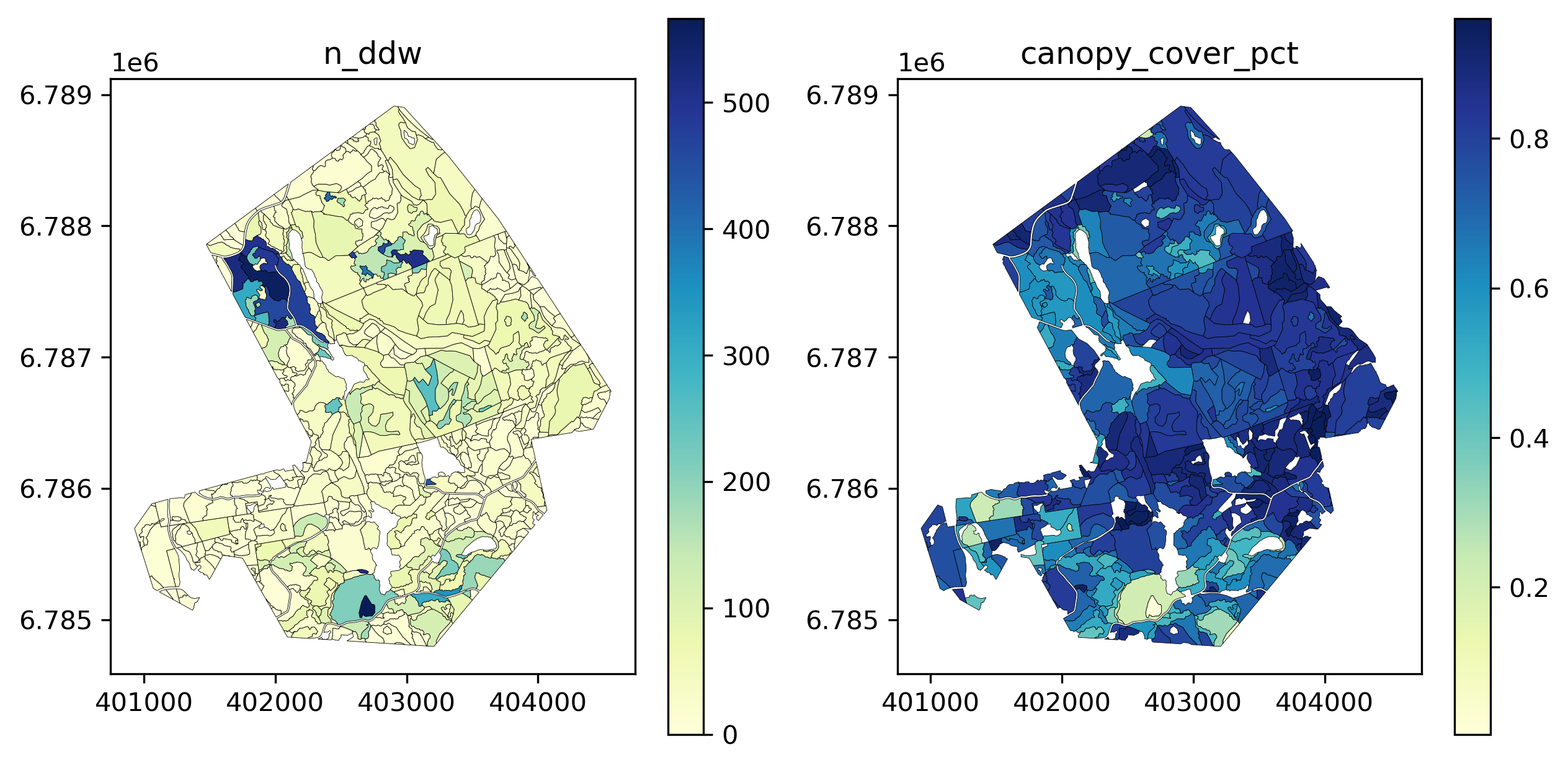

Not much, aside for perhaps the areas in the upper-central stands.

Next see effect of canopy cover and different deadwood types, separated by conservation.

Code

sns.lmplot(data=spk_stands, x='n_dw', y='canopy_cover_pct', hue='conservation', col='conservation')

<seaborn.axisgrid.FacetGrid>

Aggregated n_dw

Code

pd.pivot_table(data=spk_stands, index=['conservation'], values=['n_dw'],
               aggfunc=['min', 'max', 'mean', 'median','std', 'count'], margins=True)

	min	max	mean	median	std	count
	n_dw	n_dw	n_dw	n_dw	n_dw	n_dw
conservation
0	0.000000	631.790744	52.090442	19.745502	98.545014	381
1	3.995206	553.470919	100.909354	71.261682	103.233080	145
All	0.000000	631.790744	65.548127	29.410884	102.121836	526

Same for n_udw.

Code

sns.lmplot(data=spk_stands, x='n_udw', y='canopy_cover_pct', hue='conservation', col='conservation')

<seaborn.axisgrid.FacetGrid>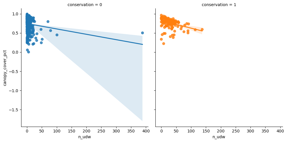

Canopy cover seems not to affect standing deadwood detections.

Code

pd.pivot_table(data=spk_stands, index=['conservation'], values=['n_udw'],
               aggfunc=['min', 'max', 'mean', 'median','std', 'count'], margins=True)

	min	max	mean	median	std	count
	n_udw	n_udw	n_udw	n_udw	n_udw	n_udw
conservation
0	0.0	388.329980	6.500767	2.411091	21.967670	381
1	0.0	137.254902	27.411903	23.857527	23.109761	145
All	0.0	388.329980	12.265244	4.077489	24.150758	526

Seems to be clear difference between conserved and managed forests, as mean values differ a lot.

Then n_ddw.

Code

sns.lmplot(data=spk_stands, x='n_ddw', y='canopy_cover_pct', hue='conservation', col='conservation')

<seaborn.axisgrid.FacetGrid>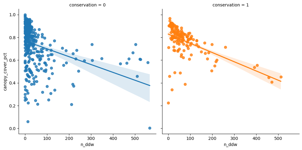

Clear-ish that denser canopy means fewer detections.

Code

pd.pivot_table(data=spk_stands, index=['conservation'], values=['n_ddw'],
               aggfunc=['min', 'max', 'mean', 'median','std', 'count'], margins=True)

	min	max	mean	median	std	count
	n_ddw	n_ddw	n_ddw	n_ddw	n_ddw	n_ddw
conservation
0	0.0	566.716642	45.589675	14.925373	90.948590	381
1	0.0	511.257036	73.497452	49.458449	86.954054	145
All	0.0	566.716642	53.282883	21.543022	90.646476	526

Conserved forests generally have more fallen deadwood instances than managed.

Then v_ddw.

Code

sns.lmplot(data=spk_stands, x='v_ddw', y='canopy_cover_pct', hue='conservation', col='conservation')

<seaborn.axisgrid.FacetGrid>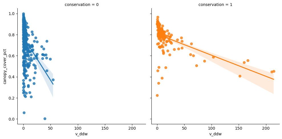

Code

pd.pivot_table(data=spk_stands, index=['conservation'], values=['v_ddw'],
               aggfunc=['min', 'max', 'mean', 'median','std', 'count'], margins=True)

	min	max	mean	median	std	count
	v_ddw	v_ddw	v_ddw	v_ddw	v_ddw	v_ddw
conservation
0	0.0	54.578953	4.757696	1.494159	8.503932	381
1	0.0	214.149358	17.851251	8.164946	35.245017	145
All	0.0	214.149358	8.367136	2.428219	20.672735	526

Difference in the estimated volume of downed deadwood per hectare between conserved and managed forests is clear.

Finally v_ddw and n_ddw:

Code

sns.lmplot(data=spk_stands, x='v_ddw', y='n_ddw', hue='conservation', col='conservation')

<seaborn.axisgrid.FacetGrid>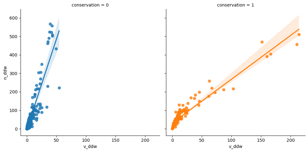

Fallen deadwood in conserved forests are clearly smaller.

2 Data aggregated to 16x16m grid

Some tasks, such as Zonation analyses, require data to be aggregated to 16x16m grid. First make that kind of grid.

Code

from itertools import product
gridsize = 16
xmin, ymin, xmax, ymax = spk_results.total_bounds
cells = []
for x, y in tqdm(product(np.arange(xmin, xmax+gridsize, gridsize),np.arange(ymin, ymax+gridsize, gridsize))):
    x1 = x - gridsize
    y1 = y + gridsize
    cells.append(box(x,y,x1,y1))

58534it [00:00, 120200.79it/s]

Then define some functions that get the information.

Code

def get_n_dw(row, trees, tree_sindex):
    nearest_idx = list(tree_sindex.nearest(row.geometry.bounds))
    tempdf = trees.iloc[nearest_idx]
    return len(tempdf[tempdf.geometry.intersects(row.geometry)])

def get_n_udw(row, trees, tree_sindex):
    nearest_idx = list(tree_sindex.nearest(row.geometry.bounds))
    tempdf = trees.iloc[nearest_idx]
    tempdf = tempdf[tempdf.layer == 'uprightwood']
    return len(tempdf[tempdf.geometry.intersects(row.geometry)])

def get_n_ddw(row, trees, tree_sindex):
    nearest_idx = list(tree_sindex.nearest(row.geometry.bounds))
    tempdf = trees.iloc[nearest_idx]
    tempdf = tempdf[tempdf.layer == 'groundwood']
    return len(tempdf[tempdf.geometry.intersects(row.geometry)])

def get_v_ddw(row, trees, tree_sindex):
    nearest_idx = list(tree_sindex.nearest(row.geometry.bounds))
    tempdf = trees.iloc[nearest_idx]
    return tempdf[tempdf.layer=='groundwood'].clip(row.geometry).v_ddw.sum()

Attach the information to grid cells.

Code

grid = gpd.GeoDataFrame(cells, columns=['geometry'], crs=spk_results.crs)
trees_sindex = spk_results.sindex
grid['n_dw'] = grid.progress_apply(lambda row: get_n_dw(row, spk_results, trees_sindex), axis=1)
grid['n_udw'] = grid.progress_apply(lambda row: get_n_udw(row, spk_results, trees_sindex), axis=1)
grid['n_ddw'] = grid.progress_apply(lambda row: get_n_ddw(row, spk_results, trees_sindex), axis=1)
grid['v_ddw'] = grid.progress_apply(lambda row: get_v_ddw(row, spk_results, 
                                                          trees_sindex), axis=1)

100%|███████████████████████████████████████████████████████████████████████████| 58534/58534 [02:26<00:00, 400.86it/s]
100%|███████████████████████████████████████████████████████████████████████████| 58534/58534 [04:48<00:00, 202.91it/s]
100%|███████████████████████████████████████████████████████████████████████████| 58534/58534 [03:20<00:00, 291.94it/s]
100%|███████████████████████████████████████████████████████████████████████████| 58534/58534 [04:14<00:00, 230.02it/s]

Plot n_dw.

Code

grid[grid.n_dw > 0].plot(column='n_dw', legend=True, figsize=(20,12), cmap='YlGnBu').set_title('n_dw in 16m grid')

Text(0.5, 1.0, 'n_dw in 16m grid')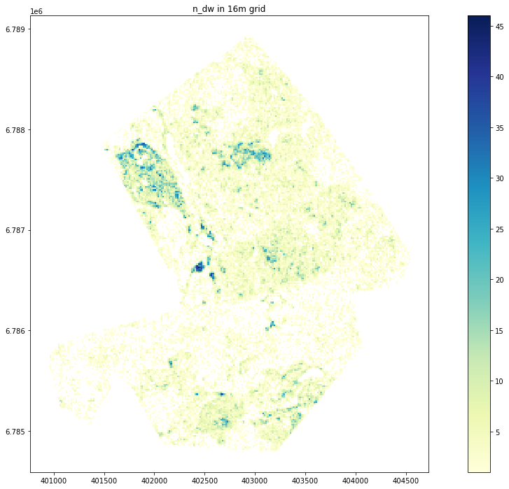

Plot n_udw

Code

grid[grid.n_udw > 0].plot(column='n_udw', legend=True, figsize=(20,12), cmap='YlGnBu').set_title('n_udw in 16m grid')

Text(0.5, 1.0, 'n_udw in 16m grid')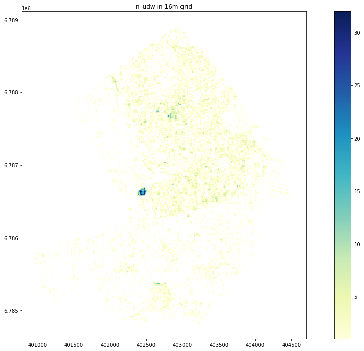

Plot n_ddw

Code

grid[grid.n_ddw > 0].plot(column='n_ddw', legend=True, figsize=(20,12), cmap='YlGnBu').set_title('n_ddw in 16m grid')

Text(0.5, 1.0, 'n_ddw in 16m grid')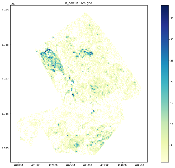

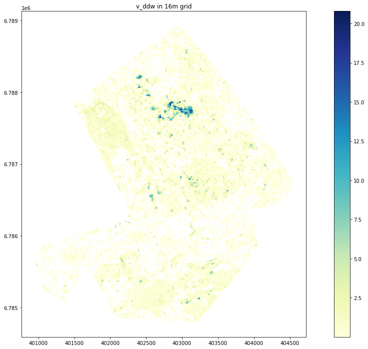
Plot v_ddw

Code

grid[(grid.v_ddw > 0)].plot(column='v_ddw', legend=True, figsize=(20,12), cmap='YlGnBu').set_title('v_ddw in 16m grid')

Text(0.5, 1.0, 'v_ddw in 16m grid')