Code
from drone_detector.utils import * from drone_detector.imports import * import rasterio.mask as rio_maskimport seaborn as sns'whitegrid' )import warnings"ignore" )'..' )from src.tree_functions import *
Here we first compare the annotations and predictions in field plot level metrics, and then do the same for predictions and field data. Comparison between annotations and predictions is done with all data within the scenes, whereas the comparisons between predictions and field data are done with the predictions intersecting the field plot circle.
Hiidenportti
Read data and do some wrangling. Hiidenportti data comparisons are done only with the five test scenes.
Code
= Path('../data/hiidenportti' )= gpd.read_file('../../data/raw/hiidenportti/virtual_plots/all_deadwood_hiidenportti.geojson' )= gpd.read_file('../results/hiidenportti/merged_all_20220823.geojson' )= gpd.read_file(field_data_path/ 'plot_circles.geojson' )= pd.read_csv(field_data_path/ 'all_plot_data.csv' )= gpd.read_file(field_data_path/ 'envelopes_with_trees.geojson' )= gpd.read_file('../data/common/LsAlueValtio.shp' )= conservation_areas[conservation_areas.geometry.intersects(box(* anns.total_bounds))]= gpd.clip(cons_hp, virtual_plot_grid)
Filter plot circles so that only those present in scenes remain.
Code
'in_vplot' ] = plot_circles.apply (lambda row: 1 if any (virtual_plot_grid.geometry.contains(row.geometry)) else 0 , axis= 1 )'id' ] = plot_circles['id' ].astype(int )= field_data[field_data.id .isin(plot_circles[plot_circles.in_vplot== 1 ].id .unique())]= {c: c.replace('.' ,'_' ) for c in field_data.columns}, inplace= True )= ['id' ] + [c for c in field_data.columns if 'dw' in c]= field_data[dw_cols].copy()= plot_circles[plot_circles.in_vplot == 1 ]
Code
= pd.read_csv(field_data_path/ 'hp_tree_data_fixed_1512.csv' )= tree_data[tree_data.plot_id.isin(plot_dw_data.id .unique())]== 'EDNA_45' ) & (tree_data.tree_class == 4 ) & (tree_data.DBH < 100 )].index, inplace= True )
Count the number of deadwood (n_dw), fallen deadwood (n_ddw) and standing deadwood (n_udw) from the individual field data measurements.
Code
'n_dw_plot' ] = plot_dw_data.id .apply (lambda row: len (tree_data[tree_data.plot_id == row]))'n_ddw_plot' ] = plot_dw_data.id .apply (lambda row: len (tree_data[(tree_data.plot_id == row) & (tree_data.tree_class == 4 )]))'n_udw_plot' ] = plot_dw_data.id .apply (lambda row: len (tree_data[(tree_data.plot_id == row) & (tree_data.tree_class == 3 )]))
Some helper functions for data matching.
Code
def match_circular_plot(row, plots):"Match annotations with field plots" for p in plots.itertuples():if row.geometry.intersects(p.geometry):return int (p.id )def match_vplot(row, plots):"Match annotations with field plots" for p in plots.itertuples():if row.geometry.intersects(p.geometry):return f' { p. id } _ { p. level_1} ' 'plot_id' ] = anns.apply (lambda row: match_circular_plot(row, plot_circles), axis= 1 )= anns.overlay(plot_circles[['geometry' ]])'plot_id' ] = anns_in_plots.plot_id.astype(int )
Add relevant information to predictions.
Code
'conservation' ] = preds.geometry.apply (lambda row: 1 if any (cons_hp.geometry.contains(row))else 0 )'plot_id' ] = preds.apply (lambda row: match_circular_plot(row, plot_circles), axis= 1 )= preds.overlay(plot_circles[['geometry' ]])'plot_id' ] = preds_in_plots.plot_id.astype(int )'vplot_id' ] = preds.apply (lambda row: match_vplot(row, virtual_plot_grid), axis= 1 )
Filter only test areas
Code
= anns_in_plots[anns_in_plots.plot_id.isin(preds_in_plots.plot_id.unique())]= plot_dw_data[plot_dw_data.id .isin(preds_in_plots.plot_id.unique())]= anns[anns.vplot_id.isin(preds.vplot_id.unique())]
Predictions vs annotations, with all data present in the scenes
First crosstab the numbers of different deadwood types. First annotations.
Code
= True )
layer
groundwood
uprightwood
All
conservation
0
916
181
1097
1
485
159
644
All
1401
340
1741
Then predictions.
Code
= True )
layer
groundwood
uprightwood
All
conservation
0
1211
373
1584
1
792
191
983
All
2003
564
2567
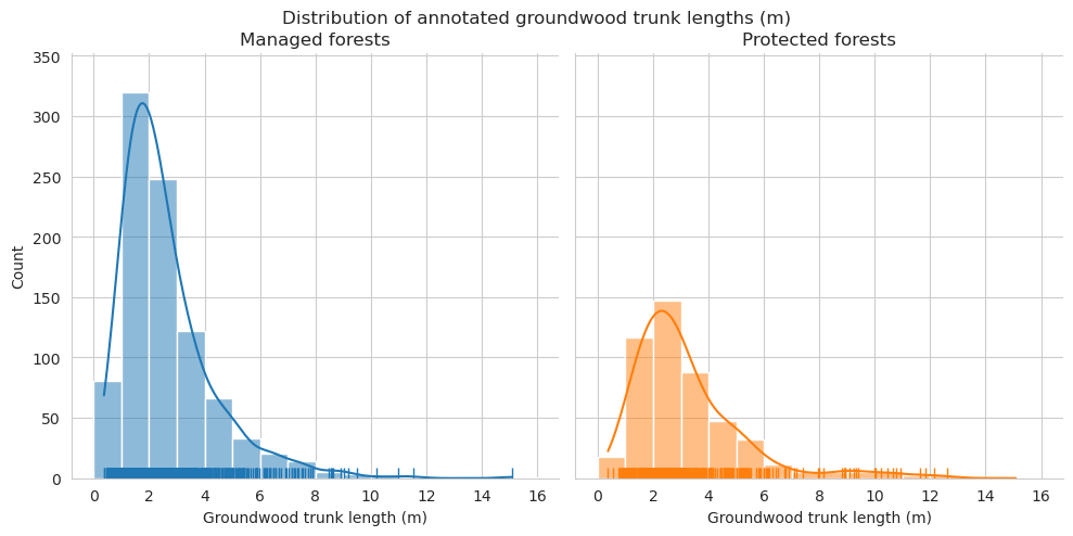
Add tree length and diameter estimations and check them for groundwood.
Code
'tree_length' ] = anns.geometry.apply (get_len)'tree_length' ] = preds.geometry.apply (get_len)'diam' ] = anns.geometry.apply (lambda row: np.mean(get_three_point_diams(row))) * 1000 'diam' ] = preds.geometry.apply (lambda row: np.mean(get_three_point_diams(row))) * 1000
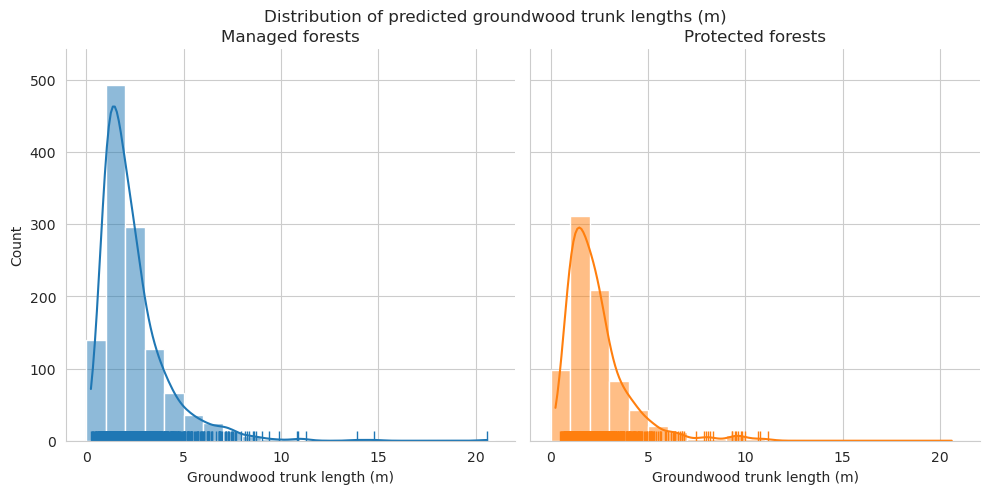
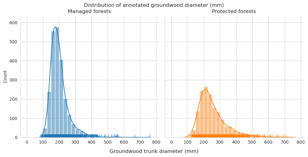
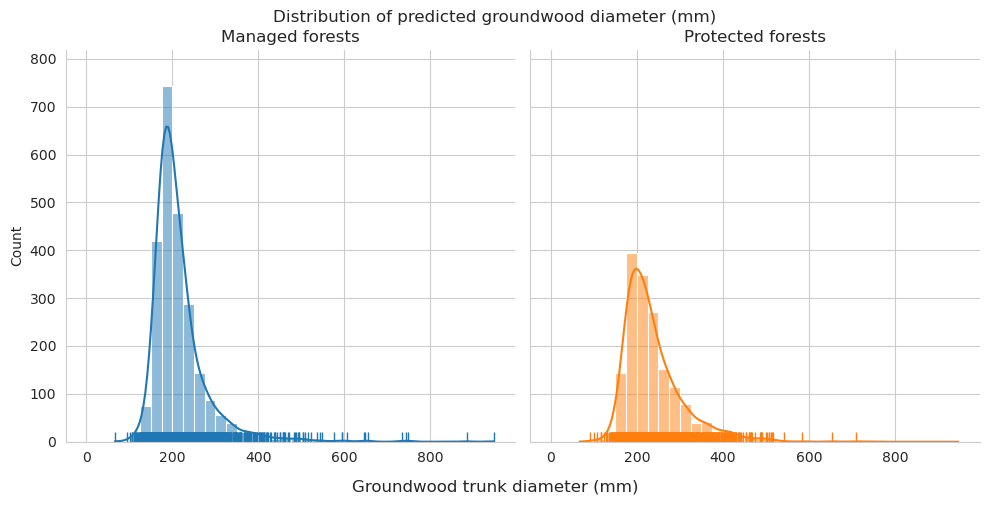
Distributions for length look pretty similar, though there are some clear outliers in the predictions.
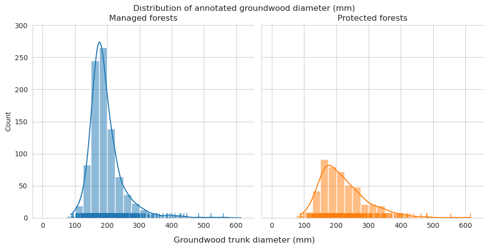
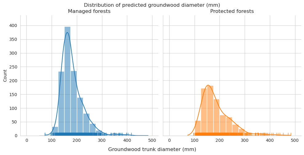
Diameter distributions differ mostly in the 150-175mm class, which is overrepresented for predictions in managed forests.
Check the statistics for diameter and length.
Code
== 'groundwood' ].pivot_table(index= 'conservation' , values= ['diam' , 'tree_length' ], = True , aggfunc= ['mean' , 'min' , 'max' ])
mean
min
max
diam
tree_length
diam
tree_length
diam
tree_length
conservation
0
194.449747
2.621222
89.906915
0.383440
558.643918
15.087245
1
220.942312
3.208590
87.563515
0.371857
614.556062
12.617573
All
203.620977
2.824558
87.563515
0.371857
614.556062
15.087245
Code
== 'groundwood' ].pivot_table(index= 'conservation' , values= ['diam' , 'tree_length' ], = True , aggfunc= ['mean' , 'min' , 'max' ])
mean
min
max
diam
tree_length
diam
tree_length
diam
tree_length
conservation
0
181.405153
2.390542
73.158266
0.234854
416.484903
20.598724
1
187.242699
2.351327
95.175610
0.472634
483.888458
11.152778
All
183.713359
2.375036
73.158266
0.234854
483.888458
20.598724
Check the area covered by standing deadwood canopies. First annotations.
Code
'area_m2' ] = anns.geometry.area'area_m2' ] = preds.geometry.area== 'uprightwood' ].pivot_table(index= 'conservation' , values= ['area_m2' ], margins= True ,= ['mean' , 'sum' ])
mean
sum
area_m2
area_m2
conservation
0
3.066763
555.084039
1
4.061288
645.744719
All
3.531849
1200.828758
Then predictions. Predictions seem to slightly underestimate the sizes of standing deadwood canopies.
Code
== 'uprightwood' ].pivot_table(index= 'conservation' , values= ['area_m2' ], margins= True ,= ['mean' , 'sum' ])
mean
sum
area_m2
area_m2
conservation
0
2.574031
960.113404
1
3.667250
700.444729
All
2.944252
1660.558133
Check the volume estimations.
Code
'v_ddw' ] = anns.geometry.apply (cut_cone_volume)'v_ddw' ] = preds.geometry.apply (cut_cone_volume)'vplot_id' ] = virtual_plot_grid.apply (lambda p: f' { p. id } _ { p. level_1} ' , axis= 1 )= cons_hp.overlay(virtual_plot_grid[virtual_plot_grid.vplot_id.isin(preds.vplot_id.unique())])= virtual_plot_grid[virtual_plot_grid.vplot_id.isin(preds.vplot_id.unique())].area.sum ()= test_cons_areas.area.sum ()= test_vplot_area - test_cons_area= test_man_area / 10000 = test_cons_area / 10000 = anns[(anns.layer== 'groundwood' )& (anns.conservation== 0 )].v_ddw.sum ()/ test_man_ha= anns[(anns.layer== 'groundwood' )& (anns.conservation== 1 )].v_ddw.sum ()/ test_cons_ha= anns[(anns.layer== 'groundwood' )].v_ddw.sum ()/ (test_vplot_area/ 10000 )= preds[(preds.layer== 'groundwood' )& (preds.conservation== 0 )].v_ddw.sum ()/ test_man_ha= preds[(preds.layer== 'groundwood' )& (preds.conservation== 1 )].v_ddw.sum ()/ test_cons_ha= preds[(preds.layer== 'groundwood' )].v_ddw.sum ()/ (test_vplot_area/ 10000 )
Code
print (f'Estimated groundwood volume in managed forests, based on annotations: { ann_est_v_man:.2f} ha/m³' )print (f'Estimated groundwood volume in conserved forests, based on annotations: { ann_est_v_cons:.2f} ha/m³' )print (f'Estimated groundwood volume in both types, based on annotations: { ann_est_v_test:.2f} ha/m³' )
Estimated groundwood volume in managed forests, based on annotations: 13.05 ha/m³
Estimated groundwood volume in conserved forests, based on annotations: 14.05 ha/m³
Estimated groundwood volume in both types, based on annotations: 13.50 ha/m³
Code
print (f'Estimated groundwood volume in managed forests, based on predictions: { pred_est_v_man:.2f} ha/m³' )print (f'Estimated groundwood volume in conserved forests, based on predictions: { pred_est_v_cons:.2f} ha/m³' )print (f'Estimated groundwood volume in both types, based on predictions: { pred_est_v_test:.2f} ha/m³' )
Estimated groundwood volume in managed forests, based on predictions: 15.02 ha/m³
Estimated groundwood volume in conserved forests, based on predictions: 13.74 ha/m³
Estimated groundwood volume in both types, based on predictions: 14.43 ha/m³
Predictions vs field data, with only predictions present in field plots
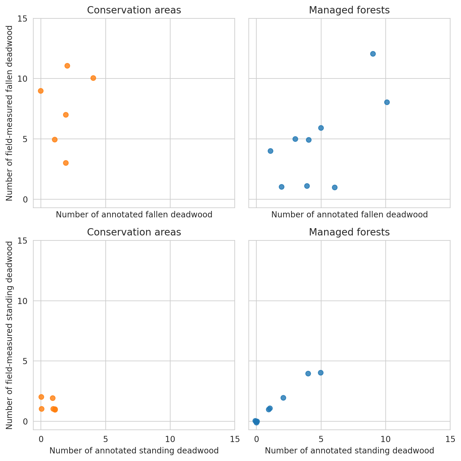
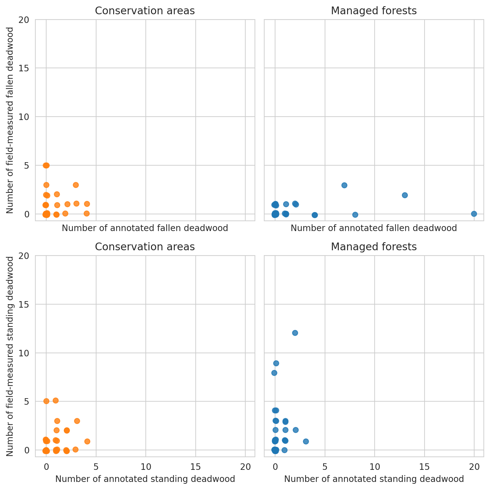
Count the number of annotated deadwood instances in each circular field plot, as well as note which of the circular plots are located in the conserved areas.
Code
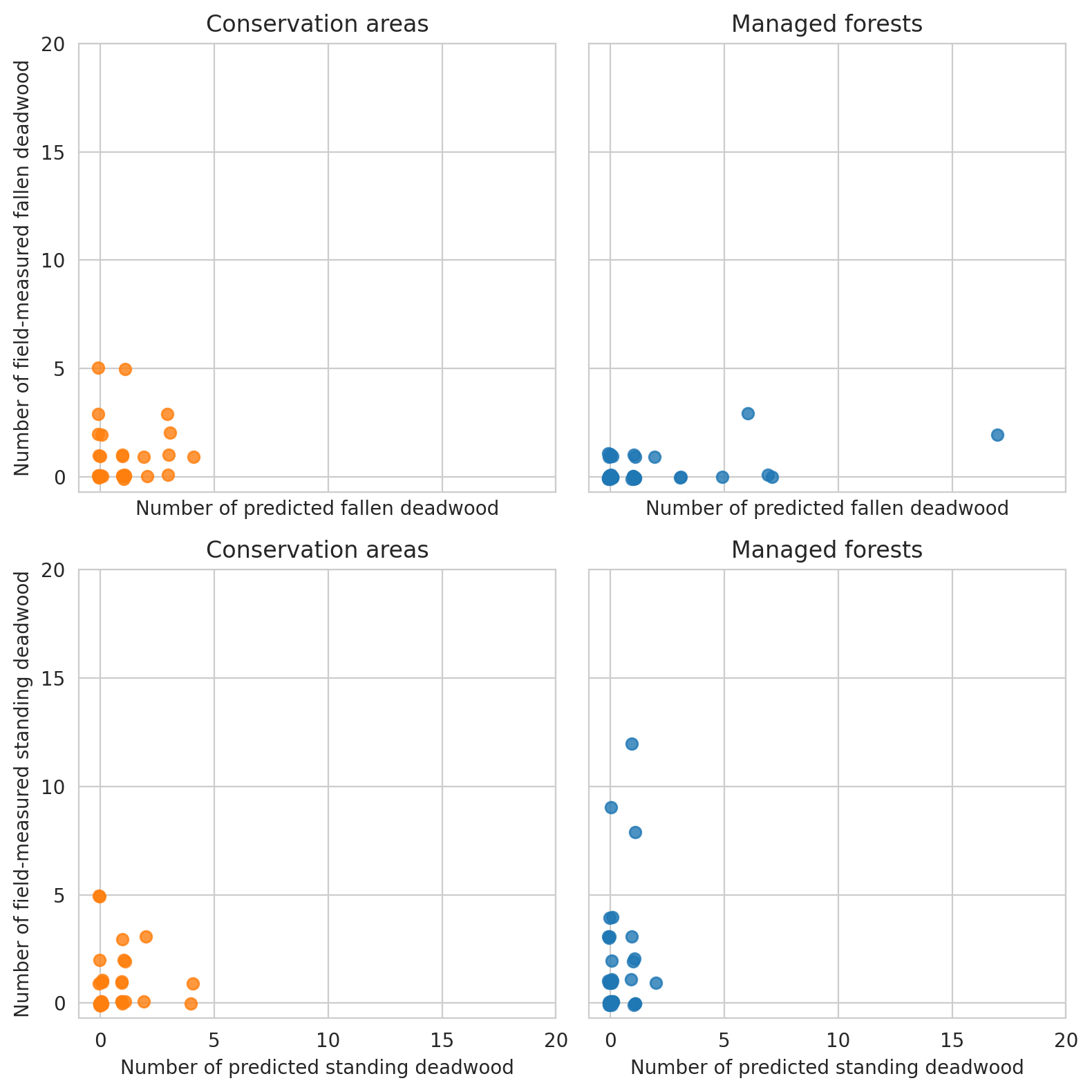
'n_dw_ann' ] = plot_dw_data.apply (lambda row: anns_in_plots.plot_id.value_counts()[row.id ] if row.id in anns_in_plots.plot_id.unique() else 0 , axis= 1 )'n_ddw_ann' ] = plot_dw_data.apply (lambda row: anns_in_plots[anns_in_plots.groundwood== 2 ].plot_id.value_counts()[row.id ] if row.id in anns_in_plots[anns_in_plots.groundwood== 2 ].plot_id.unique() else 0 , axis= 1 )'n_udw_ann' ] = plot_dw_data.apply (lambda row: anns_in_plots[anns_in_plots.groundwood== 1 ].plot_id.value_counts()[row.id ] if row.id in anns_in_plots[anns_in_plots.groundwood== 1 ].plot_id.unique() else 0 , axis= 1 )'geometry' ] = plot_dw_data.apply (lambda row: plot_circles[plot_circles.id == row.id ].geometry.iloc[0 ], = 1 )= gpd.GeoDataFrame(plot_dw_data, crs= plot_circles.crs)'conservation' ] = plot_dw_data.apply (lambda row: 1 if any (cons_hp.geometry.contains(row.geometry))else 0 , axis= 1 )'n_dw_pred' ] = plot_dw_data.apply (lambda row: preds_in_plots.plot_id.value_counts()[row.id ] if row.id in preds_in_plots.plot_id.unique() else 0 , axis= 1 )'n_ddw_pred' ] = plot_dw_data.apply (lambda row: preds_in_plots[preds_in_plots.label== 2 ].plot_id.value_counts()[row.id ] if row.id in preds_in_plots[preds_in_plots.label== 2 ].plot_id.unique() else 0 , axis= 1 )'n_udw_pred' ] = plot_dw_data.apply (lambda row: preds_in_plots[preds_in_plots.label== 1 ].plot_id.value_counts()[row.id ] if row.id in preds_in_plots[preds_in_plots.label== 1 ].plot_id.unique() else 0 , axis= 1 )
Compare the numbers of annotations (n_*_ann), predictions (n_*_pred) and field measured (n_*_plot) deadwood instances.
Code
= 'conservation' , values= ['n_ddw_plot' , 'n_udw_plot' , 'n_ddw_ann' , 'n_udw_ann' ,'n_ddw_pred' , 'n_udw_pred' ], = 'sum' , margins= True )
n_ddw_ann
n_ddw_plot
n_ddw_pred
n_udw_ann
n_udw_plot
n_udw_pred
conservation
0
44
43
57
13
12
15
1
11
45
22
4
8
3
All
55
88
79
17
20
18
Get plot-wise canopy cover percentage based on LiDAR derived canopy height model as the percentage of plot area with height more than 2 meters.
Code
= []with rio.open ('../../data/raw/hiidenportti/full_mosaics/CHM_Hiidenportti_epsg.tif' ) as src:= src.crsfor row in plot_dw_data.itertuples():= rio_mask.mask(src, [row.geometry], crop= True )> 2 ].shape[0 ] / plot_im[plot_im >= 0 ].shape[0 ])'canopy_cover_pct' ] = pcts
Plot the relationship between annotated deadwood and field data.
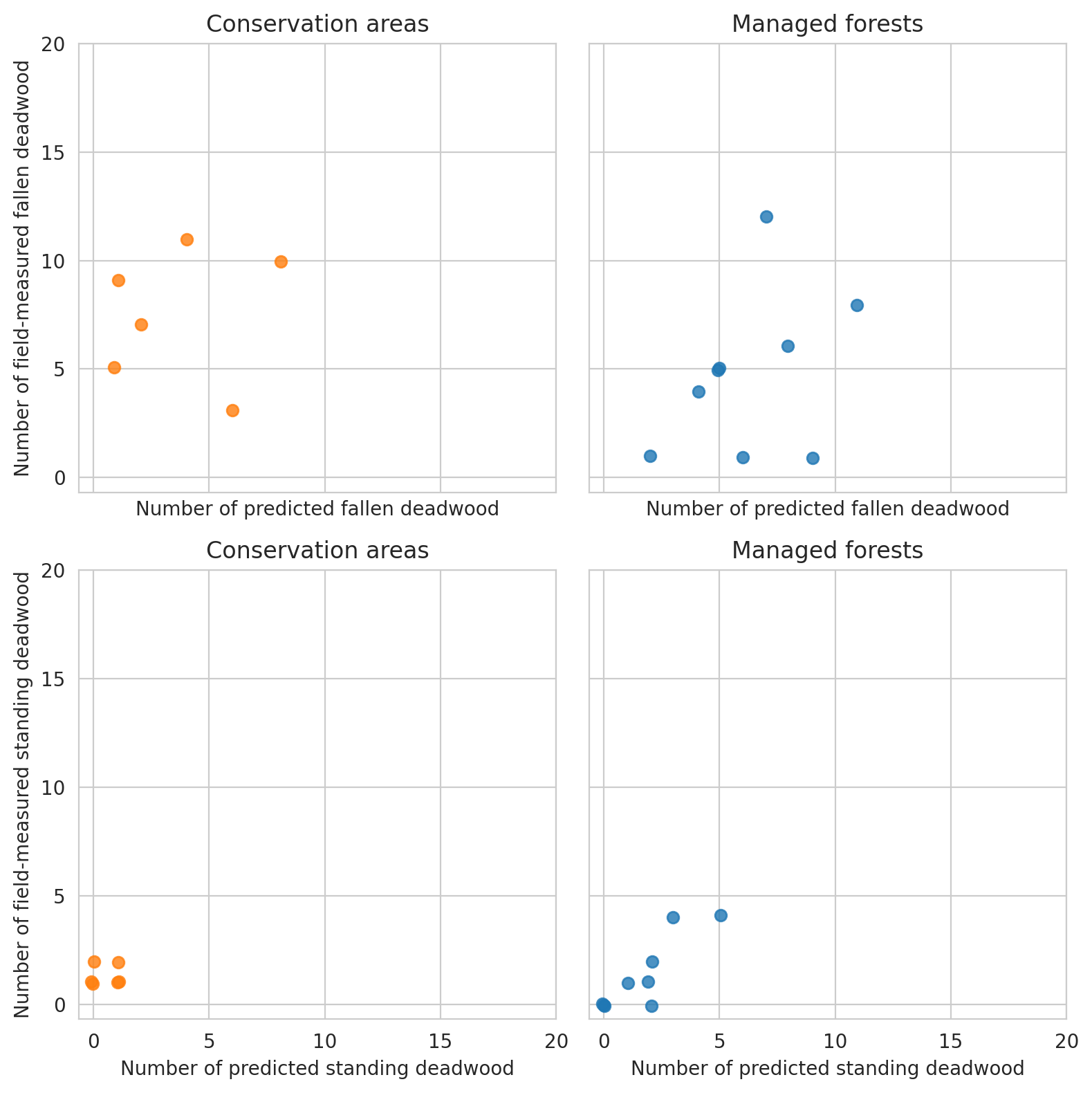
Same for field data and predictions
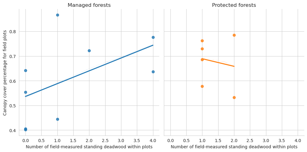
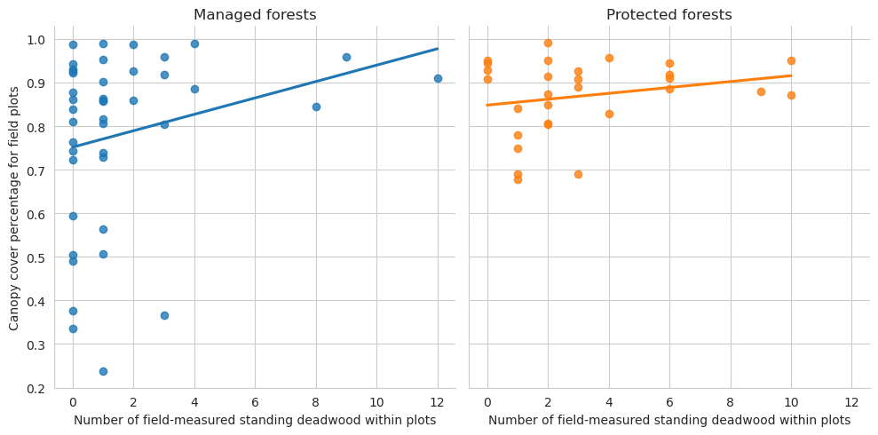
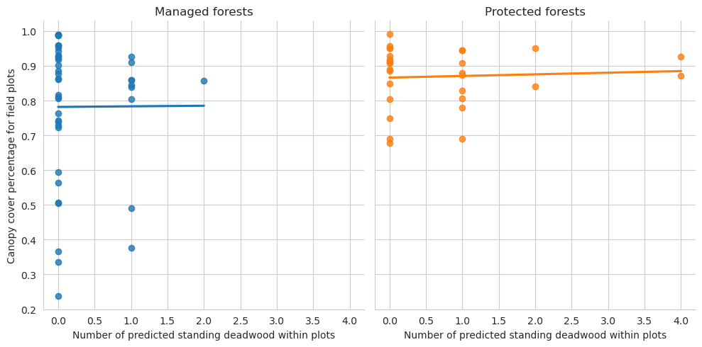
Next the relationship between canopy cover and types of detected deadwood.
Code
= sns.lmplot(data= plot_dw_data, x= 'n_udw_plot' , y= 'canopy_cover_pct' , col= 'conservation' , hue= 'conservation' , ci= 1 ,= False )0 ,0 ].set_title('Managed forests' )0 ,1 ].set_title('Protected forests' )'Canopy cover percentage for field plots' )'Number of field-measured standing deadwood within plots' )
Code
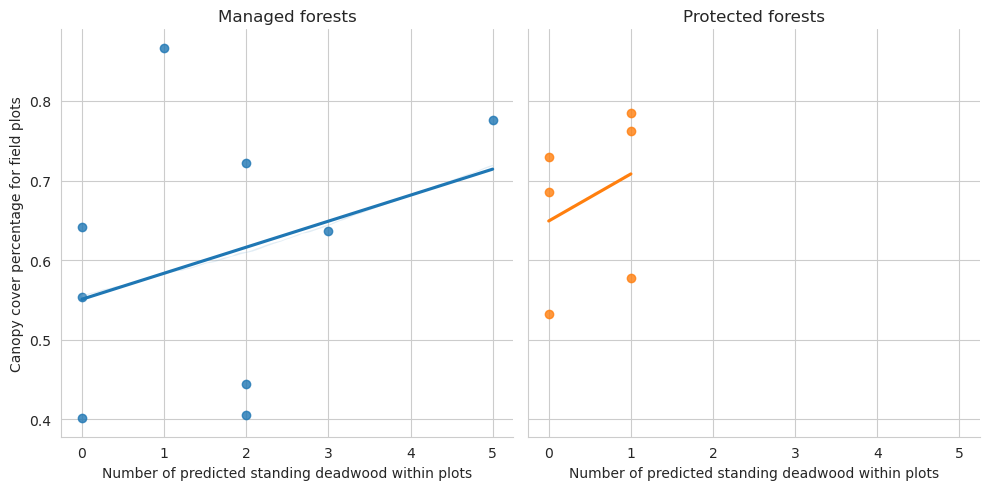
= sns.lmplot(data= plot_dw_data, x= 'n_udw_pred' , y= 'canopy_cover_pct' , col= 'conservation' , hue= 'conservation' , ci= 1 ,= False )0 ,0 ].set_title('Managed forests' )0 ,1 ].set_title('Protected forests' )'Canopy cover percentage for field plots' )'Number of predicted standing deadwood within plots' )
Code
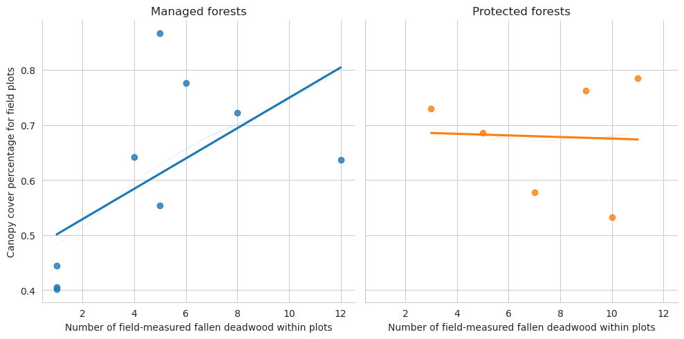
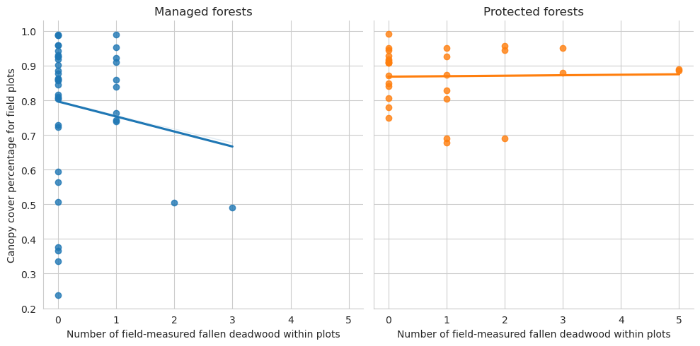
= sns.lmplot(data= plot_dw_data, x= 'n_ddw_plot' , y= 'canopy_cover_pct' , col= 'conservation' , hue= 'conservation' , ci= 1 ,= False )0 ,0 ].set_title('Managed forests' )0 ,1 ].set_title('Protected forests' )'Canopy cover percentage for field plots' )'Number of field-measured fallen deadwood within plots' )
Code
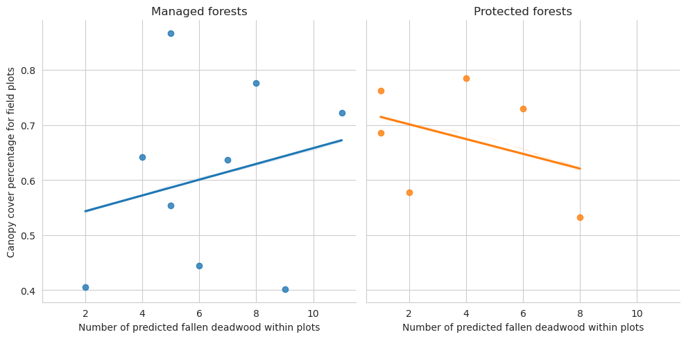
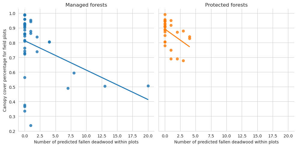
= sns.lmplot(data= plot_dw_data, x= 'n_ddw_pred' , y= 'canopy_cover_pct' , col= 'conservation' , hue= 'conservation' , ci= 1 ,= False )0 ,0 ].set_title('Managed forests' )0 ,1 ].set_title('Protected forests' )'Canopy cover percentage for field plots' )'Number of predicted fallen deadwood within plots' )
Note that for the test set there are too few plots to draw meaningful conclusions.
Add information about conservation area to tree data.
Code
= tree_data[tree_data.plot_id.isin(plot_dw_data.id .unique())]'conservation' ] = tree_data.apply (lambda row: plot_dw_data[plot_dw_data.id == row.plot_id].conservation.unique()[0 ], axis= 1 )'conservation' ] = preds_in_plots.apply (lambda row: plot_dw_data[plot_dw_data.id == row.plot_id].conservation.unique()[0 ], axis= 1 )'tree_length' ] = anns_in_plots.apply (lambda row: get_len(row.geometry), axis= 1 )'tree_length' ] = preds_in_plots.apply (lambda row: get_len(row.geometry), axis= 1 )
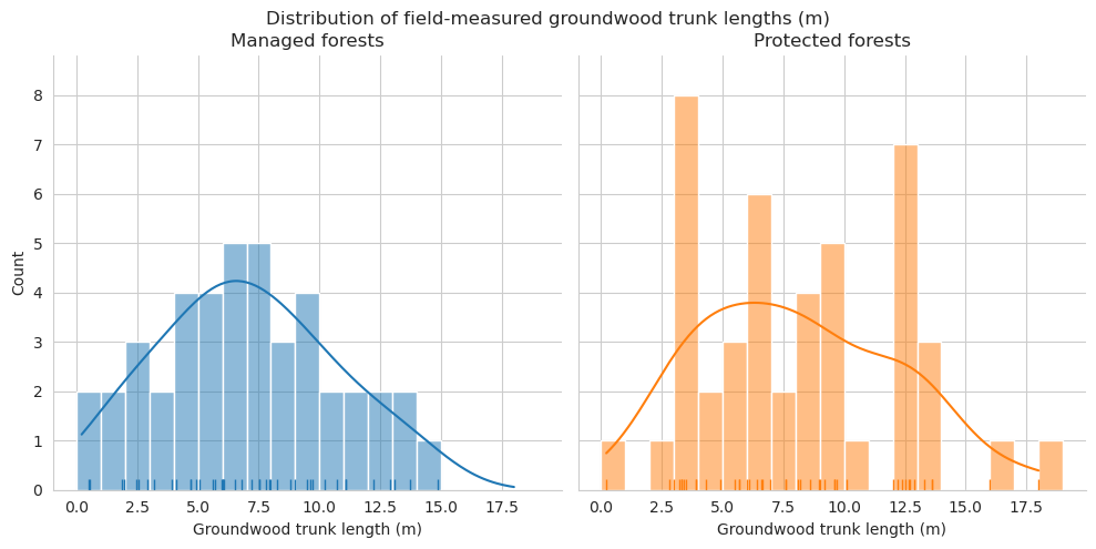
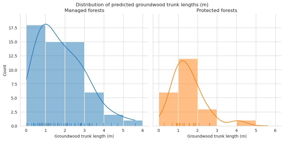
Compare the distributions of the downed trunk lengths. Both graphs only take the parts within the plots into account. Lengths are binned into 1m bins.
As expected, annotated trunks are clearly on average shorter than field measured.
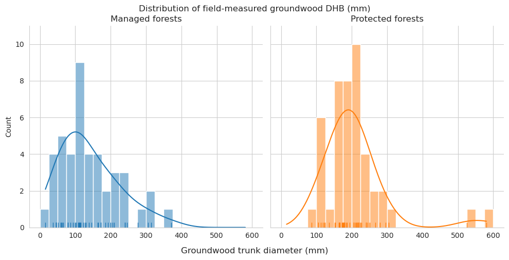
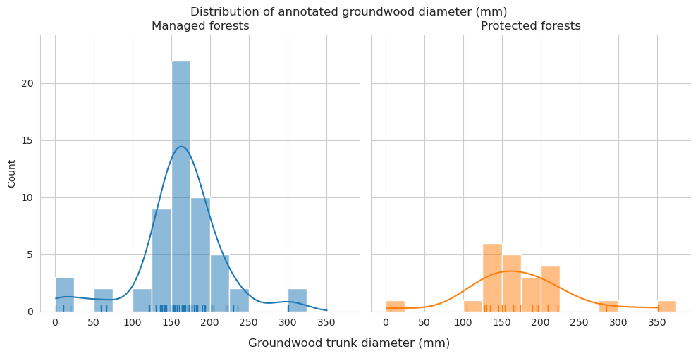
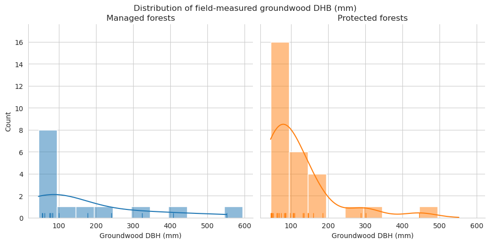
Compare the measured DBH for downed trees and estimated diameter of annotated downed deadwood. For annotated deadwood, the diameter is estimated for the whole tree, not only for the part within the field plot. DBHs are binned into 50mm bins.
See the statistics for groundwood length and diameter. First for field data.
Code
= tree_data[(tree_data.tree_class == 4 )& (tree_data.DBH> 0 )],= ['conservation' ], values= ['l' , 'DBH' ],= ['mean' , 'min' , 'max' ], margins= True )
mean
min
max
DBH
l
DBH
l
DBH
l
conservation
0
140.100016
7.040370
15.558197
0.518478
371.498790
14.855550
1
206.043641
8.075359
86.112222
0.214113
580.560964
18.000666
All
173.821188
7.569625
15.558197
0.214113
580.560964
18.000666
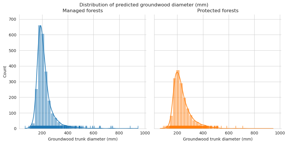
Then for predictions.
Code
= preds_in_plots[(preds_in_plots.label== 2 )& (preds_in_plots.tree_length >= 0.1 )], = ['conservation' ], values= ['tree_length' , 'diam' ],= ['mean' , 'min' , 'max' ], margins= True )
mean
min
max
diam
tree_length
diam
tree_length
diam
tree_length
conservation
0
166.508194
1.889520
10.889255
0.281128
301.422460
5.605036
1
172.456022
1.524233
6.250000
0.285395
350.669633
4.077773
All
168.207574
1.785152
6.250000
0.281128
350.669633
5.605036
Then compare the statistics for volume estimations, first for field data.
Code
'v_ddw' ] = anns_in_plots.geometry.apply (cut_cone_volume)'v_ddw_ann' ] = plot_dw_data.apply (lambda row: anns_in_plots[(anns_in_plots.plot_id == row.id ) & == 'groundwood' )sum ()= 1 )'v_ddw' ] = preds_in_plots.geometry.apply (cut_cone_volume)'v_ddw_pred' ] = plot_dw_data.apply (lambda row: preds_in_plots[(preds_in_plots.plot_id == row.id ) & == 'groundwood' )sum ()= 1 )'v_dw_plot' ] = (plot_dw_data['v_dw' ]/ 10000 )* np.pi* 9 ** 2 'v_ddw_plot' ] = (plot_dw_data['v_ddw' ]/ 10000 )* np.pi* 9 ** 2 'v_udw_plot' ] = plot_dw_data.v_dw_plot - plot_dw_data.v_ddw_plot= plot_dw_data, index= ['conservation' ], values= ['v_ddw' ],= ['min' , 'max' , 'mean' , 'median' ,'std' , 'count' ], margins= True )
min
max
mean
median
std
count
v_ddw
v_ddw
v_ddw
v_ddw
v_ddw
v_ddw
conservation
0
1.476682
88.948335
29.528714
22.513292
28.686318
9
1
65.155283
139.171786
82.494768
71.816212
28.298432
6
All
1.476682
139.171786
50.715136
48.100161
38.439837
15
Then for predictions.
Code
'v_ddw_pred_ha' ] = (10000 * plot_dw_data.v_ddw_pred) / (np.pi * 9 ** 2 )= plot_dw_data, index= ['conservation' ], values= ['v_ddw_pred_ha' ],= ['min' , 'max' , 'mean' , 'median' ,'std' , 'count' ], margins= True )
min
max
mean
median
std
count
v_ddw_pred_ha
v_ddw_pred_ha
v_ddw_pred_ha
v_ddw_pred_ha
v_ddw_pred_ha
v_ddw_pred_ha
conservation
0
4.239953
24.857178
13.098547
11.497471
8.527684
9
1
0.515183
30.041972
7.896543
3.257221
11.360618
6
All
0.515183
30.041972
11.017745
6.405077
9.726651
15
Based on these plots, our predictions clearly underestimate the total volume of fallen deadwood, especially in conserved forests.
Sudenpesänkangas
Read data and do some wrangling.
Code
= Path('../data/sudenpesankangas/' )= gpd.read_file('../../data/raw/sudenpesankangas/virtual_plots/sudenpesankangas_deadwood.geojson' )= evo_anns.to_crs('epsg:3067' )= gpd.read_file('../results/sudenpesankangas/spk_merged_20220825.geojson' )= gpd.read_file(evo_fd_path/ 'plot_circles.geojson' )'id' ] = evo_plot_circles['id' ].astype(int )= pd.read_csv(evo_fd_path/ 'puutiedot_sudenpesänkangas.csv' , sep= ';' , decimal= ',' )= gpd.GeoDataFrame(evo_field_data, geometry= gpd.points_from_xy(evo_field_data.gx, evo_field_data.gy), = 'epsg:3067' )= gpd.read_file(evo_fd_path/ 'vplots.geojson' )= evo_grid.to_crs('epsg:3067' )'plotid' ] = evo_field_data.kaid + 1000 = evo_field_data[evo_field_data.puuluo.isin([3 ,4 ])]= conservation_areas[conservation_areas.geometry.intersects(box(* evo_anns.total_bounds))]= gpd.clip(cons_evo, evo_grid)def match_plotid_spk(geom, plots):for r in plots.itertuples():if r.geometry.intersects(geom):return r.id return None def match_vplot_spk(geom, plots):for p in plots.itertuples():if geom.intersects(p.geometry):return f' { p. fid} _ { int (p.id )} '
Get up-to-date field data
Code
= pd.read_csv(evo_fd_path/ 'Koealatunnukset_Evo_2018.txt' , sep= ' ' )= pd.read_csv(evo_fd_path/ 'Koealatunnukset_Evo_2018_LUKE.txt' , sep= ' ' )= gpd.GeoDataFrame(evo_plots_updated, geometry= gpd.points_from_xy(evo_plots_updated.x,= 'epsg:3067' )= gpd.GeoDataFrame(evo_plots_luke, geometry= gpd.points_from_xy(evo_plots_luke.x,= 'epsg:3067' )= pd.concat([evo_plots_updated, evo_plots_luke])= {c: c.replace('.' ,'_' ) for c in evo_plots.columns}, inplace= True )'spk_id' ] = evo_plots.geometry.apply (lambda row: match_plotid_spk(row, evo_plot_circles))= 'spk_id' , inplace= True )'geometry' ] = evo_plots.spk_id.apply (lambda row: evo_plot_circles[evo_plot_circles.id == row].geometry.iloc[0 ])= ['id' ], inplace= True )= {'spk_id' : 'id' }, inplace= True )'conservation' ] = evo_plots.geometry.apply (lambda row: 1 if cons_evo.geometry.unary_union.intersects(row)else 0 )'plot_id' ] = evo_anns.apply (lambda row: int (row.vplot_id.split('_' )[1 ]), axis= 1 )= evo_plots[evo_plots.id .isin(evo_anns.plot_id.unique())]'plot_id' ] = evo_anns.apply (lambda row: match_circular_plot(row, evo_plots), axis= 1 )= evo_anns.overlay(evo_plots[['geometry' ]])'conservation' ] = evo_preds.geometry.apply (lambda row: 1 if any (cons_evo.geometry.contains(row))else 0 )'vplot_id' ] = evo_preds.geometry.apply (lambda row: match_vplot_spk(row, evo_grid))'plot_id' ] = evo_preds.apply (lambda row: match_circular_plot(row, evo_plots), axis= 1 )= evo_preds.overlay(evo_plots[['geometry' ]])'plot_id' ] = evo_preds_in_plots.plot_id.astype(int )
Predictions vs annotations, all available data
Compare the numbers, first annotations.
Code
= True )
label
groundwood
uprightwood
All
conservation
0
2369
386
2755
1
1546
1033
2579
All
3915
1419
5334
Then predictions.
Code
= True )
layer
groundwood
uprightwood
All
conservation
0
2437
383
2820
1
1693
807
2500
All
4130
1190
5320
Add lenght and diameter information to groundwood.
Code
'tree_length' ] = evo_anns.geometry.apply (get_len)'tree_length' ] = evo_preds.geometry.apply (get_len)'diam' ] = evo_anns.geometry.apply (lambda row: np.mean(get_three_point_diams(row))) * 1000 'diam' ] = evo_preds.geometry.apply (lambda row: np.mean(get_three_point_diams(row))) * 1000
The clearest difference between these distributions are that on average the predictions are shorter than annotations.
Then statistics for groundwood diameter and length. First annotations.
Code
== 'groundwood' ].pivot_table(index= 'conservation' , values= ['diam' , 'tree_length' ], = True , aggfunc= ['mean' , 'min' , 'max' ])
mean
min
max
diam
tree_length
diam
tree_length
diam
tree_length
conservation
0
200.474161
3.113435
85.977992
0.605847
760.781151
24.479043
1
254.250328
3.914179
101.096059
0.575351
709.170305
22.625422
All
221.709909
3.429642
85.977992
0.575351
760.781151
24.479043
Then predictions. On average, predictions are both shorter and thinner than annotations.
Code
== 'groundwood' ].pivot_table(index= 'conservation' , values= ['diam' , 'tree_length' ], = True , aggfunc= ['mean' , 'min' , 'max' ])
mean
min
max
diam
tree_length
diam
tree_length
diam
tree_length
conservation
0
215.721066
2.285198
66.289676
0.281653
946.777021
14.455624
1
237.056243
2.832194
90.435975
0.251623
710.128841
18.956571
All
224.466939
2.509427
66.289676
0.251623
946.777021
18.956571
Check area covered by standing deadwood canopies. First annotations.
Code
'area_m2' ] = evo_anns.geometry.area'area_m2' ] = evo_preds.geometry.area== 'uprightwood' ].pivot_table(index= 'conservation' , values= ['area_m2' ], margins= True ,= ['mean' , 'sum' ])
mean
sum
area_m2
area_m2
conservation
0
3.142462
1212.990283
1
5.811285
6003.057735
All
5.085305
7216.048018
Then predictions. On average predicted canopies are larger than annotated.
Code
== 'uprightwood' ].pivot_table(index= 'conservation' , values= ['area_m2' ], margins= True ,= ['mean' , 'sum' ])
mean
sum
area_m2
area_m2
conservation
0
3.750448
1436.421535
1
5.776561
4661.684400
All
5.124459
6098.105935
Code
'v_ddw' ] = evo_anns.geometry.apply (cut_cone_volume)'v_ddw' ] = evo_preds.geometry.apply (cut_cone_volume)= evo_grid.area.sum ()= cons_evo.area.sum ()= evo_vplot_area - evo_cons_area= evo_man_area / 10000 = evo_cons_area / 10000 = evo_anns[(evo_anns.label== 'groundwood' )& (evo_anns.conservation== 0 )].v_ddw.sum ()/ evo_man_ha= evo_anns[(evo_anns.label== 'groundwood' )& (evo_anns.conservation== 1 )].v_ddw.sum ()/ evo_cons_ha= evo_anns[(evo_anns.label== 'groundwood' )].v_ddw.sum ()/ (evo_vplot_area/ 10000 )= evo_preds[(evo_preds.layer== 'groundwood' )& (evo_preds.conservation== 0 )].v_ddw.sum ()/ evo_man_ha= evo_preds[(evo_preds.layer== 'groundwood' )& (evo_preds.conservation== 1 )].v_ddw.sum ()/ evo_cons_ha= evo_preds[(evo_preds.layer== 'groundwood' )].v_ddw.sum ()/ (evo_vplot_area/ 10000 )
Code
print (f'Estimated groundwood volume in managed forests, based on annotations: { evo_ann_est_v_man:.2f} ha/m³' )print (f'Estimated groundwood volume in conserved forests, based on annotations: { evo_ann_est_v_cons:.2f} ha/m³' )print (f'Estimated groundwood volume in both types, based on annotations: { evo_ann_est_v:.2f} ha/m³' )
Estimated groundwood volume in managed forests, based on annotations: 7.08 ha/m³
Estimated groundwood volume in conserved forests, based on annotations: 13.97 ha/m³
Estimated groundwood volume in both types, based on annotations: 9.90 ha/m³
Code
print (f'Estimated groundwood volume in managed forests, based on predictions: { evo_pred_est_v_man:.2f} ha/m³' )print (f'Estimated groundwood volume in conserved forests, based on predictions: { evo_pred_est_v_cons:.2f} ha/m³' )print (f'Estimated groundwood volume in both types, based on predictions: { evo_pred_est_v:.2f} ha/m³' )
Estimated groundwood volume in managed forests, based on predictions: 7.03 ha/m³
Estimated groundwood volume in conserved forests, based on predictions: 10.17 ha/m³
Estimated groundwood volume in both types, based on predictions: 8.31 ha/m³
Predictions vs field data, plot-wise
Add canopy density based on LiDAR derived canopy height model. The density is the percentage of field plot area with height above 2 meters.
Code
= []with rio.open ('../../data/raw/sudenpesankangas/full_mosaics/sudenpesankangas_chm.tif' ) as src:for row in evo_plots.itertuples():= rio_mask.mask(src, [row.geometry], crop= True )> 2 ].shape[0 ] / plot_im[plot_im >= 0 ].shape[0 ])'canopy_cover_pct' ] = pcts= evo_plots, index= ['conservation' ], values= ['canopy_cover_pct' ],= ['min' , 'max' , 'mean' , 'std' , 'count' ], margins= True )
min
max
mean
std
count
canopy_cover_pct
canopy_cover_pct
canopy_cover_pct
canopy_cover_pct
canopy_cover_pct
conservation
0
0.237288
0.989960
0.782452
0.200439
42
1
0.678000
0.991992
0.869878
0.085901
29
All
0.237288
0.991992
0.818162
0.168393
71
Count the number of deadwood instances similarly as for Hiidenportti data and plot the relationship between them.
Code
'n_dw_ann' ] = evo_plots.apply (lambda row: evo_anns.plot_id.value_counts()[int (row.id )]if row.id in evo_anns.plot_id.unique() else 0 , axis= 1 )'n_ddw_ann' ] = evo_plots.apply (lambda row: evo_anns[evo_anns.label== 'groundwood' ].plot_id.value_counts()[int (row.id )]if row.id in evo_anns[evo_anns.label== 'groundwood' ].plot_id.unique() else 0 , axis= 1 )'n_udw_ann' ] = evo_plots.apply (lambda row: evo_anns[evo_anns.label!= 'groundwood' ].plot_id.value_counts()[int (row.id )]if row.id in evo_anns[evo_anns.label!= 'groundwood' ].plot_id.unique() else 0 , axis= 1 )'n_dw_plot' ] = np.round ((evo_plots['n_dw' ]/ 10000 )* np.pi* 9 ** 2 ).astype(int )'n_ddw_plot' ] = np.round ((evo_plots['n_ddw' ]/ 10000 )* np.pi* 9 ** 2 ).astype(int )'n_udw_plot' ] = evo_plots.n_dw_plot - evo_plots.n_ddw_plot'conservation' ] = evo_plots.apply (lambda row: 1 if any (cons_evo.geometry.contains(row.geometry))else 0 , axis= 1 )'n_dw_pred' ] = evo_plots.apply (lambda row: evo_preds.plot_id.value_counts()[int (row.id )]if row.id in evo_preds.plot_id.unique() else 0 , axis= 1 )'n_ddw_pred' ] = evo_plots.apply (lambda row: evo_preds[evo_preds.layer== 'groundwood' ].plot_id.value_counts()[int (row.id )]if row.id in evo_preds[evo_preds.layer== 'groundwood' ].plot_id.unique() else 0 , axis= 1 )'n_udw_pred' ] = evo_plots.apply (lambda row: evo_preds[evo_preds.layer!= 'groundwood' ].plot_id.value_counts()[int (row.id )]if row.id in evo_preds[evo_preds.layer!= 'groundwood' ].plot_id.unique() else 0 , axis= 1 )
Compare the number of annotations, predictions and field measurements within plots.
Code
= 'conservation' , values= ['n_ddw_plot' , 'n_udw_plot' , 'n_ddw_ann' , 'n_udw_ann' , 'n_ddw_pred' , 'n_udw_pred' ], = 'sum' , margins= True )
n_ddw_ann
n_ddw_plot
n_ddw_pred
n_udw_ann
n_udw_plot
n_udw_pred
conservation
0
65
14
59
14
68
11
1
22
29
30
29
92
21
All
87
43
89
43
160
32
Plot the relationship between annotated and field data.
Same for field data and predictions.
Relationship between canopy cover and deadwood.
Code
= sns.lmplot(data= evo_plots, x= 'n_udw_plot' , y= 'canopy_cover_pct' , col= 'conservation' , hue= 'conservation' , ci= 1 ,= False )0 ,0 ].set_title('Managed forests' )0 ,1 ].set_title('Protected forests' )'Canopy cover percentage for field plots' )'Number of field-measured standing deadwood within plots' )
Code
= sns.lmplot(data= evo_plots, x= 'n_udw_pred' , y= 'canopy_cover_pct' , col= 'conservation' , hue= 'conservation' , ci= 1 ,= False )0 ,0 ].set_title('Managed forests' )0 ,1 ].set_title('Protected forests' )'Canopy cover percentage for field plots' )'Number of predicted standing deadwood within plots' )
Code
= sns.lmplot(data= evo_plots, x= 'n_ddw_plot' , y= 'canopy_cover_pct' , col= 'conservation' , hue= 'conservation' , ci= 1 ,= False )0 ,0 ].set_title('Managed forests' )0 ,1 ].set_title('Protected forests' )'Canopy cover percentage for field plots' )'Number of field-measured fallen deadwood within plots' )
Code
= sns.lmplot(data= evo_plots, x= 'n_ddw_ann' , y= 'canopy_cover_pct' , col= 'conservation' , hue= 'conservation' , ci= 1 ,= False )0 ,0 ].set_title('Managed forests' )0 ,1 ].set_title('Protected forests' )'Canopy cover percentage for field plots' )'Number of predicted fallen deadwood within plots' )
As Evo data doesn’t have field-measured deadwood lengths, we can’t plot that relationship. We can, however, plot the DBH distributions, even though Evo dataset only has around 50 downed deadwood with dbh measured.
Code
= evo_field_data[evo_field_data.plotid.isin(evo_plots.id .unique())]'conservation' ] = evo_field_data.apply (lambda row: evo_plots[evo_plots.id == row.plotid].conservation.unique()[0 ], axis= 1 )
est_pituus_m is the estimated lenght of the deadwood, based on DBH (lapimitta_mm) and growth formulae, so that is really inaccurate.
Code
= evo_field_data[(evo_field_data.puuluo == 4 )& (evo_field_data.lapimitta_mm> 0 )],= ['conservation' ], values= ['est_pituus_m' , 'lapimitta_mm' ],= ['mean' , 'min' , 'max' , 'count' ], margins= True )
mean
min
max
count
est_pituus_m
lapimitta_mm
est_pituus_m
lapimitta_mm
est_pituus_m
lapimitta_mm
est_pituus_m
lapimitta_mm
conservation
0
13.609571
169.357143
5.934
55
34.211
552
14
14
1
11.905690
115.896552
5.446
45
28.101
445
29
29
All
12.460442
133.302326
5.446
45
34.211
552
43
43
Length and diameter statistics for predictions.
Code
'tree_length' ] = evo_preds_in_plots.geometry.apply (get_len)= evo_preds_in_plots[evo_preds_in_plots.label== 2 ], index= ['conservation' ], = ['tree_length' , 'diam' ],= ['mean' , 'min' , 'max' ], margins= True )
mean
min
max
diam
tree_length
diam
tree_length
diam
tree_length
conservation
0
215.914297
1.962542
69.619593
0.375545
502.915702
9.128894
1
211.666849
2.007725
74.672309
0.242613
356.577743
6.525554
All
214.482573
1.977772
69.619593
0.242613
502.915702
9.128894
Estimated volume statistics for Evo area. First based on field data.
Code
'v_ddw' ] = evo_preds_in_plots.geometry.apply (cut_cone_volume)'v_ddw_pred' ] = evo_plots.apply (lambda row: evo_preds_in_plots[(evo_preds_in_plots.plot_id == row.id ) & == 'groundwood' )sum ()= 1 )'v_ddw_pred_ha' ] = (10000 * evo_plots.v_ddw_pred) / (np.pi * 9 ** 2 )= evo_plots, index= ['conservation' ], values= ['v_ddw' ],= ['min' , 'max' , 'mean' , 'median' ,'std' , 'count' ], margins= True )
min
max
mean
median
std
count
v_ddw
v_ddw
v_ddw
v_ddw
v_ddw
v_ddw
conservation
0
0.0
123.004587
5.522673
0.0
23.497052
42
1
0.0
98.258093
6.338610
0.0
18.873961
29
All
0.0
123.004587
5.855943
0.0
21.587804
71
Then based on predictions.
Code
= evo_plots, index= ['conservation' ], values= ['v_ddw_pred_ha' ],= ['min' , 'max' , 'mean' , 'median' ,'std' , 'count' ], margins= True )
min
max
mean
median
std
count
v_ddw_pred_ha
v_ddw_pred_ha
v_ddw_pred_ha
v_ddw_pred_ha
v_ddw_pred_ha
v_ddw_pred_ha
conservation
0
0.0
66.098826
5.599320
0.000000
13.330675
42
1
0.0
32.592807
4.048691
1.193922
6.801761
29
All
0.0
66.098826
4.965964
0.000000
11.098662
71